An analysis of cortical magnification data across 8 subjects.

Introduction

In this post, I explore the concept of cortical magnification using a custom dataset from the Winawer lab, in which 8 subjects were shown 12 scans each of colorful retinotopic mapping stimuli.

Retinotopy

A retinotopic map refers to the layout of one half of the visual field on the cortical surface in a manner that topologically preserves the layout of the retina.

Retinotopic maps have a consistent layout across individuals with many visual areas. These visual areas tile the occipital cortex, each containing a retinotopic map. The following shows the group-average retinotopic mapping data from the Human Connectome Project.

Cortical Magnification

The visual field must be warped in order to be mapped onto the cortical surface because the cortical surface is not flat but curved and complex. This transformation additionally biases certain parts of the visual field by allocating more of the cortex to them than other parts.

The measure of how much of the cortex is devoted to how much of the visual field is called cortical magnification. It generally has units similar to mm/deg or mm mm\(^2\)/deg\(^2\). A representation of how the warping of cortical magnification is expected to look on cortex (in V1) is shown in the following image.

Cortical magnification is known to decrease with eccentricity in V1 according to the following formula by Horton and Hoyt (1991):

where \(m\) and \(\rho\) are the mm/deg of cortical magnification and deg of eccentricity, respectively. For reference, this particular cortical magnification prediction, were it absolutely true, might look like the following images when plotted.

Data

Cortical magnification was calculated either on a per-face basis (i.e., using each face of the cortical surface) or by using path-based metrics in which a path is drawn over a small patch of cortex and the cortical surface length of the path is divided by the visual field path-length. Paths were drawn both radially (along iso-angular lines across a particular point) or tangentially (along iso-eccentric lines across a particular point). Per-face magnification was calculated in both radial and tangential directions as well, and averaged around particular points for display.

Average Cortical Magnification

Path-based Calculations

Method

Path-based calculations are computed by drawing a path on the visual field, projecting that path back onto the white cortical surface, calculating the length of each, and dividing the length of the surface-path by the length of the visual-field-path. The path can be a line along an iso-angular ray (i.e., a radial path) or along an iso-eccentric curve (i.e., a tangential path). The results below were calculated by finding the path-based cortical magnification along very small paths in the visual field; the paths were drawn radially and tangentially between points in a grid in which eccentricity values were exponentially-spaced. defined by the following code:

import numpy as np

grid_angles = np.arange(0, 181, 3)
# ==> array([  0,   3,   6,   9,  12,  15, ... 177, 180])
grid_eccens = 0.625 * (2 ** np.arange(0, 4.3, 0.075))
# ==> array([ 0.625,  0.658,  0.693,  0.730,   ... 11.487, 12.100])

This gives 58 eccentricity values and 61 polar angle points. Paths were drawn either between eccentricity points along the average inter-grid polar angle value (for radial lines) or between polar angle points along the average inter-grid eccentricity value (for tangential curves); in other words, iso-angle lines were drawn along polar angles 1.5, 4.5, 7.5, 10.5, etc. and between eccentricities (0.625, 0.658), (0.658, 0.693), (0.693, 0.730), etc. while iso-eccentric lines were drawn along eccentricities 0.642, 0.0.676, 0.712, etc.

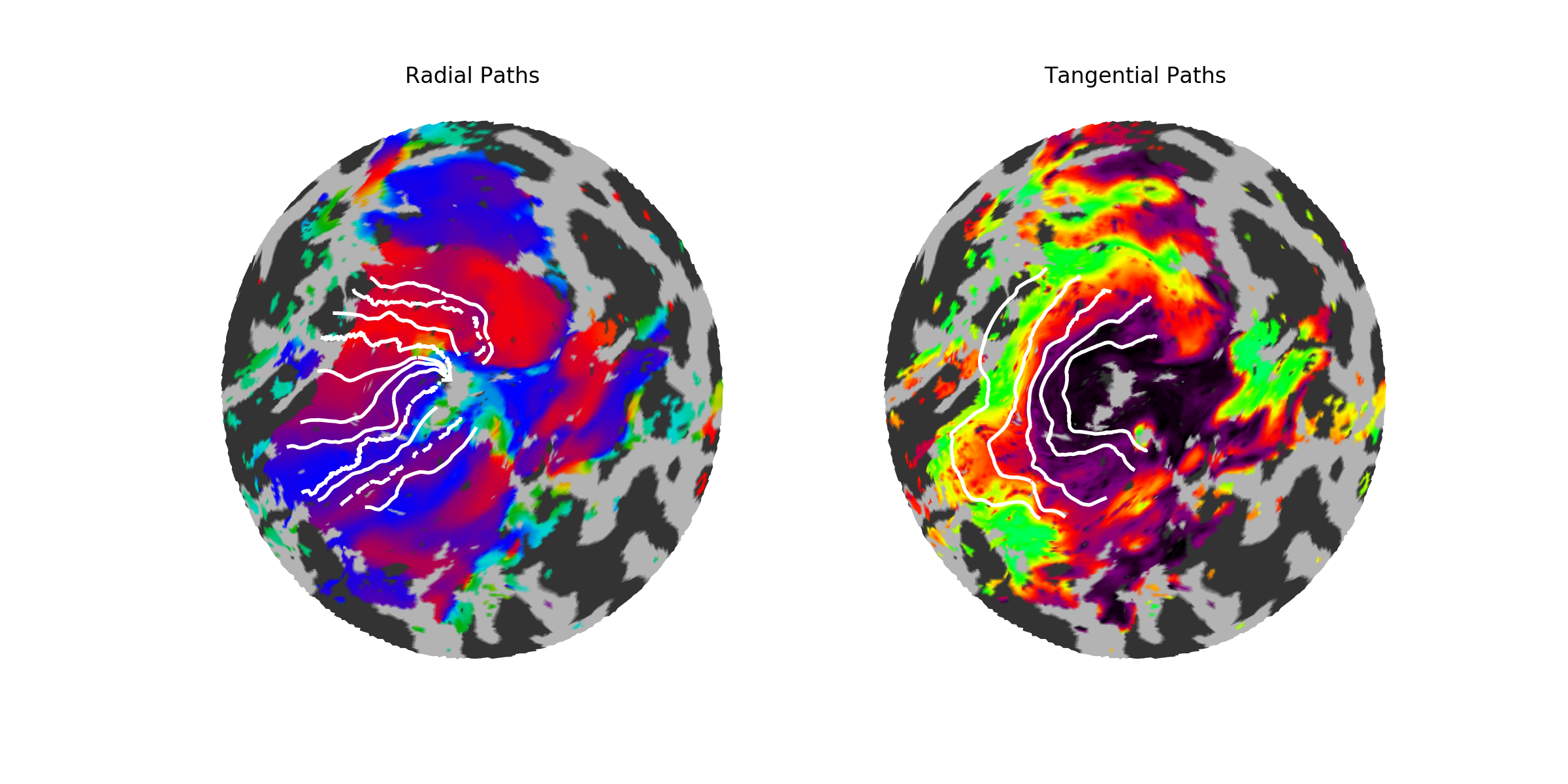
Validation. As a quick validation of the path-based cortical magnification, we can start by looking at the actual paths drawn on the cortical surface; they should resemble a best-guess as to where the iso-angle (radial) or iso-eccentric (tangential) curve should be in the validation data. If they do not, we should be skeptical of this method. The figures below show a couple example subjects; on these subjects, iso-angle lines are drawn at 0, 45, 90, 135, and 180 degrees of polar angle, except in V3 where the 0 and 180 degree lines are difficult to find, and iso-eccentricity lines are drawn at 1.5, 3. 6, and 12 degrees of eccentricity.

Subject	Left Hemisphere	Right Hemisphere
S1204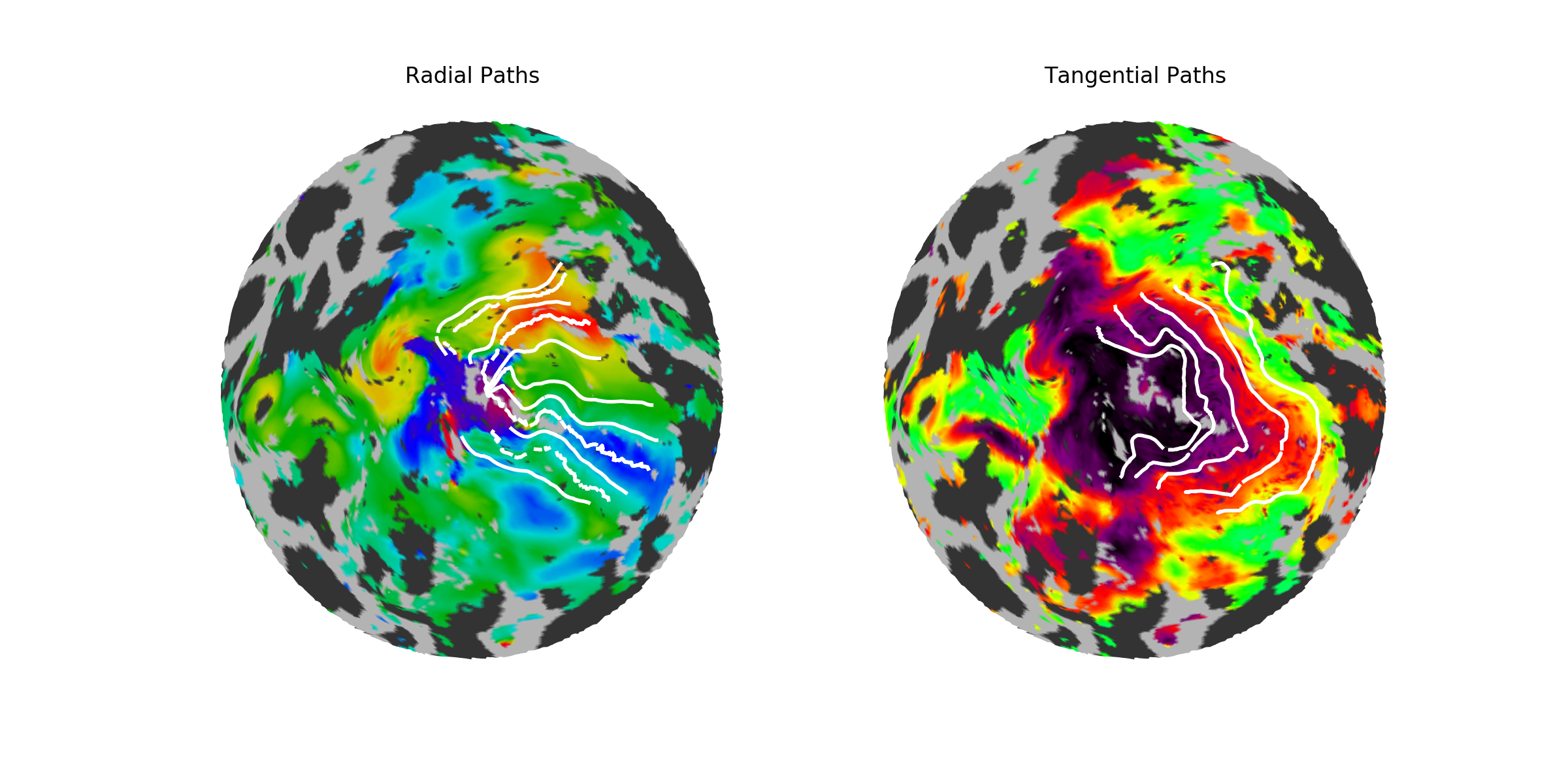
S1205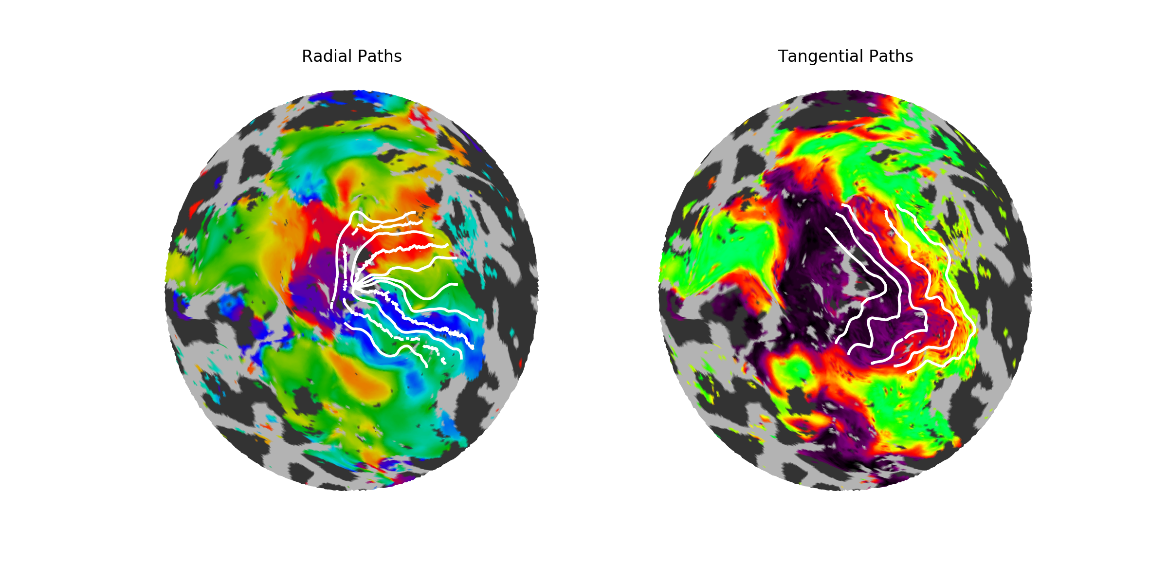

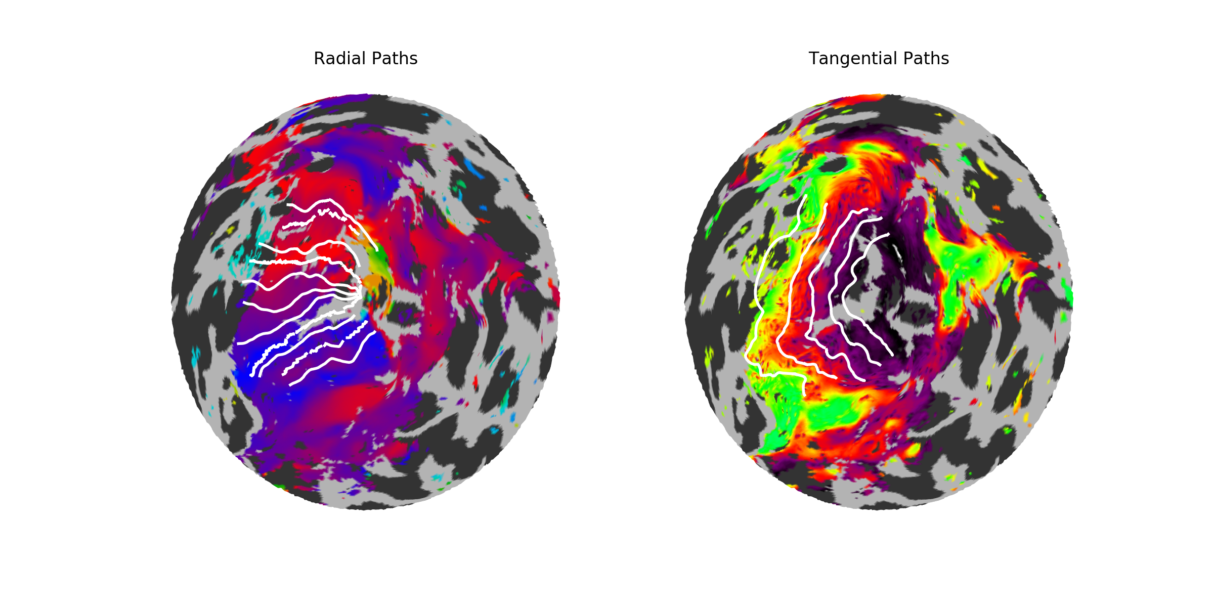These two subjects have fairly well-drawn paths. Note that a theme of these subjects and the inferred retinotopic map fits specifically (the “inferred retinotopic map fits” are not shown, but they are the maps inferred by Bayesian inference on which the paths are based) is that the dorsal V3 is often somewhat confused; many subjects have a patchy V3, and this patchiness gets represented in both the model and the individual fits. Despite this, the paths look at least fairly iso-angular, and in fact match the prescribed angles quite well.

Results

The following image shows the cortical magnification for path-based calculations; note that the dotted black lines show the 1.5, 3, and 6 degree iso-eccentricity lines, and the entire field is shown out to 12 degrees (note that there is a logarithmic scaling to eccentricity). The left images show the radial and the right images show the tangential magnification. The size of the circles is related to confidence: smaller circles have higher standard deviations across subjects (though this is not emphasized as standard deviations were generally small, except near the meridia).

If we simply collapse across polar angle values, we find that (in V1, especially) the cortical magnification values we observe from path-based calculations strongly agree with the calculations reported in Horton and Hoyt (1991).

Per-face Calculations

The following image shows the cortical magnification for per-face calculations; (see blurb in above section on path-based calculations for plot details).

As is immediately obvious from these plots, the per-face calculations are much noisier than the path-based calculations. This is probably due to the fact that the per-face measurements are dependent on many small-scale accuracies; for example, we generally expect some amount of inaccuracy in the tesselation of the FreeSurfer mesh: triangles that form the cortical surface may not be exactly the right size, and some of these triangles may have very small areas due to mesh smoothing and other sacrifices made by the tesselation algorithm. If the bias in triangle and vertex placements are relatively uniform, then we would expect paths to generate relatively uniform results because they are drawn across many triangles. One might expect the same to occur with with per-face calculations because the points in the above plots are the averages of many triangles, but this isn’t observed.

One reason for the noise in the per-face calculations despite averaging is that a single triangle whose vertices are close together can get assigned very similar visual field positions by our model because the model does not try to account for cortical magnification between vertices explicitly. (Even worse, when performing per-face calculations over raw non-inferred data, two vertices might be assigned identical visual field values from the same voxel.) When this occurs, the visual field distance is very small so the ratio of cortical surface distance to visual field distance becomes very large. The neighboring triangle might make up for this in a path-based calculation, but when we merely average a low-magnification and a high-magnification triangle, we still get an unusually high magnification. In other words, averaging the ratios is not the right way to do the per-face calculation.