MRI Data Representation and Geometry

An introduction to the representation of data and geometry in neuroscience MRI.

Introduction
File Formats
- Cortical Volumes (EPIs and Anatomical Images)
  - Voxel Data
  - Meta-Data
    - Accessing Meta-Data
    - MRImage Geometry
- Cortical Surfaces
Alignments
Interpolation

Introduction

MRI data is usually discussed as if analyzing it were the most natural thing in the world. In reality, however, the alignment of volumes and the interpolation of data between representations is only simple in theory. Similarly, the storage of surface data is usually opaque and unintuitive. This post describes the fundamentals of geometry as it applies to MRI brain data with an emphasis on FreeSurfer.

This post is not intended as a theoretical treatment of any of the issues below; rather, it is a practical guide to understanding how one’s neuroscience data is represented and to performing certain basic data transformations.

File Formats

(Back to Top)

All volume-based formats store 3D or 4D arrays of voxels in some fashion with a variety of additional meta-data. Anatomical images are typically 3D while EPIs are typically 4D (x,y,z, and time).

Cortical Volumes (EPIs and Anatomical Images)

(Back to Top)

Volumes are typically stored in one of a few ways:

DICOM (.dcm) files are the de-facto standard for MRI machines in most cases; the format is somewhat involved and is documented fully here (though I don’t suggest trying to learn the format from this page.) Though some of the meta-data in dicom files is not always transferable to other formats, it’s usually preferable not to operate on dicom files directly during data analysis.
NifTI (.nii or .nii.gz) files were created by the NIH as a solution to a previous file format called ANALYZE that was widely seen as problematic. These files are probably the most commonly used format for sharing/distributing MRI data as of when this post was written. They are usually gzipped (.nii.gz) in order to save space. The NifTI standard has a few versions, but most libraries and programs that read one will read all, and I’ve rarely if ever encountered issues with the NifTI version of a file. The NifTI header allows one to store a variety of meta-data that are most important for data analysis.
MGH (.mgh or .mgz) files are essentially FreeSurfer’s version of the NifTI file; the formats are fairly similar, at least within the perspective of the scope of this post. MGH files are typically gzipped (.mgz) to save space much like NifTI files.
Other formats, like ANALYZE, don’t appear very often in my experience, and are beyond the scope of this post.

All volume files contain both meta-data and voxels. The meta-data is just a set of information about the file’s contents while the voxels are a 3D or 4D array of values.

Voxel Data

(Back to Top)

The voxels in NifTI and MGH files are always organized into a 3D or 4D rectangular array. The various libraries for reading MGH and NifTI files automatically organize this data for you. These examples show how to access a file’s voxel array using various libraries.

Python (using nibabel)

import nibabel                      as nib
import nibabel.freesurfer.mghformat as mgh
  
# MGH/MGZ files
mgh_file = mgh.load('/Volumes/server/Freesurfer_subjects/wl_subj042/mri/brain.mgz')
mgh_file.get_data().shape
#=> (256, 256, 256)
type(mgh_file.get_data())
#=> numpy.ndarray

# NifTI files
nii_file = nib.load('/Volumes/server/Freesurfer_subjects/ernie/mri/ribbon.nii.gz')
nii_file.get_data().shape
#=> (256, 256, 256)
type(nii_file.get_data())
#=> numpy.ndarray

Python (using neuropythy, which wraps nibabel)

import neuropythy as ny
  
sub = ny.freesurfer_subject('wl_subj042')
sub.images['brain'].shape
#=> (256, 256, 256)
type(sub.images['brain'])
#=> numpy.ndarray

Matlab

addpath(genpath('/Applications/freesurfer/matlab')); % (FS installation dir on Mac)
  
mgh = MRIread('/Volumes/server/Freesurfer_subjects/wl_subj042/mri/brain.mgz');
size(mgh.vol)
%
% ans =
% 
%     256   256   256
%
class(mgh.vol)
%
% ans =
% 
%     'double'
  
tbUse vistasoft;
% ...
  
nii = niftiRead('/Volumes/server/Freesurfer_subjects/ernie/mri/ribbon.nii.gz');
size(nii.data)
% 
% ans =
% 
%    256   256   256
%
class(nii.data)
% 
%   ans =
% 
%       'uint8'
% 

Mathematica (using Neurotica)

<<Neurotica`
  
mghFile = Import[
  "/Volumes/server/Freesurfer_subjects/wl_subj042/mri/brain.mgz",
  {"GZIP", "MGH"}];
Dimensions@ImageData[mghFile]
(*=> {256, 256, 256} *)
ArrayQ[ImageData[mghFile], 3, NumericQ]
(*=> True *)
  
niiFile = Import[
  "/Volumes/server/Freesurfer_subjects/ernie/mri/ribbon.nii.gz",
  {"GZIP", "NifTI"}];
Dimensions@ImageData[niiFile]
(*=> {256, 256, 256} *)
ArrayQ[ImageData[niiFile], 3, NumericQ]
(*=> True *)

Meta-Data

(Back to Top)

A quick and easy way to examine an MRI volume file is by using the command mri_info from FreeSurfer; this command understands most MRI file formats and prints about a page of meta-data from the requested file. Here’s an example.

> mri_info /Volumes/server/Freesurfer_subjects/bert/mri/brain.mgz

Volume information for /Volumes/server/Freesurfer_subjects/bert/mri/brain.mgz
          type: MGH
    dimensions: 256 x 256 x 256
   voxel sizes: 1.0000, 1.0000, 1.0000
          type: UCHAR (0)
           fov: 256.000
           dof: 1
        xstart: -128.0, xend: 128.0
        ystart: -128.0, yend: 128.0
        zstart: -128.0, zend: 128.0
            TR: 0.00 msec, TE: 0.00 msec, TI: 0.00 msec, flip angle: 0.00 degrees
       nframes: 1
      PhEncDir: UNKNOWN
ras xform present
     xform info: x_r =  -1.0000, y_r =   0.0000, z_r =   0.0000, c_r =     5.3997
               : x_a =   0.0000, y_a =   0.0000, z_a =   1.0000, c_a =    18.0000
               : x_s =   0.0000, y_s =  -1.0000, z_s =   0.0000, c_s =     0.0000

 talairach xfm : /Volumes/server/Freesurfer_subjects/bert/mri/transforms/talairach.xfm
 Orientation   : LIA
Primary Slice Direction: coronal

voxel to ras transform:
               -1.0000   0.0000   0.0000   133.3997
                0.0000   0.0000   1.0000  -110.0000
                0.0000  -1.0000   0.0000   128.0000
                0.0000   0.0000   0.0000     1.0000

voxel-to-ras determinant -1

ras to voxel transform:
               -1.0000   0.0000   0.0000   133.3997
               -0.0000  -0.0000  -1.0000   128.0000
               -0.0000   1.0000  -0.0000   110.0000
                0.0000   0.0000   0.0000     1.0000

There’s a lot of information here, not all of which is in the scope of this post. Here are a few of the most important pieces of information:

type (MGH) just tells us the file format.
dimensions (256 x 256 x 256) tells us the number of voxels in each dimension. FreeSurfer volumes usually have the size \(256 \times 256 \times 256\) as in this example.
voxel sizes (1.0000, 1.0000, 1.0000) tells us the thickness of the voxels in each direction. Here we see that the voxels are 1 mm\(^3\) in size, but EPIs often have differently sized voxels or voxels that are not isotropic (e.g., \(1.5 \times 2 \times 2\) mm\(^3\)).
type (UCHAR (0)) refers to kind of value stored in each voxel; in most formats (MGH and NifTI) this can be a variety of sizes of integers or floating-point numbers. UCHAR means unsigned character, which is a misleading name (derived from an outdated precedent in C) for a single byte that can be between 0 and 255. Usually, for volumes containing parameters or measurements, this type will be a 32 or 64 byte floating-point value; for labels these will be integers.
fov and dof, as well as TR, TE, TI, flip angle, and PhEncDir, are all parameters related to MRI aquisition and are beyond the scope of this post.
xstart/xend, ystart/yend, and zstart/zend tell us how FreeSurfer interprets the voxels in this volume as a 3D coordinate system (more on this later).
nframes tells us the number of frames in a 4D volume. Frames are almost always stored in the volume as the last (4th) dimension.
three transformations appear in the output in the form of \(4\times 4\) matrices; we will discuss these shortly transformations shortly.
Orientation (LIA) and primary slice direction (coronal) tell us roughly how the volume is organized (more about this below also).

Note that the above values are not the only meta-data in an MGH file, and NifTI files have a slightly different set of meta-data that includes things like fields to specify the intent of the data (examples of intents: time-series data, parameters data, shape data). Full documentation of the meta-data in these formats is beyond the scope of this post, but you can read more about MGH file headers here and more about NifTI file headers here. That latter link is a well-commented C header-file; for a more human-readable explanation, try here.

Accessing Meta-Data

(Back to Top)

Another good way to look at the meta-data in a volume file is to load it with the relevant programming environment and examine the data-structures there. Here are a few examples.

Python (using nibabel)

import nibabel                      as nib
import nibabel.freesurfer.mghformat as mgh
  
# MGH/MGZ files
mgh_file = mgh.load('/Volumes/server/Freesurfer_subjects/wl_subj042/mri/brain.mgz')
mgh_file.header['dims']
#=> array([256, 256, 256,   1], dtype=int32)
mgh_file.header.get_affine()
#=> array([[-1.00000000e+00, -1.16415322e-10,  0.00000000e+00,  1.32361809e+02],
#=>        [ 0.00000000e+00, -1.90266292e-09,  9.99999940e-01, -9.83241651e+01],
#=>        [ 0.00000000e+00, -9.99999940e-01,  2.23371899e-09,  1.30323082e+02],
#=>        [ 0.00000000e+00,  0.00000000e+00,  0.00000000e+00,  1.00000000e+00]])
  
# NifTI files
nii_file = nib.load('/Volumes/server/Freesurfer_subjects/ernie/mri/ribbon.nii.gz')
nii_file.header['datatype']
#=> array(2, dtype=int16)
# (Note: the header data loaded by Nibabel are quite unprocessed and opaque)

Python (using neuropythy, which wraps nibabel)

import neuropythy as ny
  
sub = ny.freesurfer_subject('wl_subj042')
sub.mgh_images['brain'].header['dims']
#=> array([256, 256, 256,   1], dtype=int32)
sub.voxel_to_native_matrix
#=> array([[-1.00000000e+00, -1.16415322e-10,  0.00000000e+00,  1.32361809e+02],
#=>        [ 0.00000000e+00, -1.90266292e-09,  9.99999940e-01, -9.83241651e+01],
#=>        [ 0.00000000e+00, -9.99999940e-01,  2.23371899e-09,  1.30323082e+02],
#=>        [ 0.00000000e+00,  0.00000000e+00,  0.00000000e+00,  1.00000000e+00]])

# NifTI files
nii_file = ny.load('/Volumes/server/Freesurfer_subjects/ernie/mri/ribbon.nii.gz')
nii_file.header['datatype']
#=> array(2, dtype=int16)
# (Note: ny.load detects the nifti-file extension and calls nibabel.load)

Matlab

addpath(genpath('/Applications/freesurfer/matlab')); % (FS installation dir on Mac)
  
mgh = MRIread('/Volumes/server/Freesurfer_subjects/wl_subj042/mri/brain.mgz');
mgh.volres
%
% ans =
% 
%     1.0000    1.0000    1.0000
%
mgh.vox2ras
%
% ans =
% 
%    -1.0000   -0.0000         0  132.3618
%          0   -0.0000    1.0000  -98.3242
%          0   -1.0000    0.0000  130.3231
%          0         0         0    1.0000
%
%   % Note that this is the same matrix as in Python, just rounded better
  
tbUse vistasoft;
% ...
  
nii = niftiRead('/Volumes/server/Freesurfer_subjects/ernie/mri/ribbon.nii.gz');
nii.dim
% 
% ans =
% 
%    256   256   256
%

Mathematica (using Neurotica)

<<Neurotica`
  
mghFile = Import[
  "/Volumes/server/Freesurfer_subjects/wl_subj042/mri/brain.mgz",
  {"GZIP", "MGH"}];
Options[mghFile, VoxelDimensions]
(*=> {1., 1., 1.} *)
  
niiFile = Import[
  "/Volumes/server/Freesurfer_subjects/ernie/mri/ribbon.nii.gz",
  {"GZIP", "NifTI"}];
Options[niiFile, VoxelDimensions]
(*=> {1., 1., 1.} *)

MRImage Geometry

(Back to Top)

Consider the following problem: I give you a T1-weighted MR image of a subject and ask you to tell me if you think the subject’s left hemisphere occipital cortex is unusually large. You open the file and see something that looks like this:

example_volume

Looking at this, you might conclude that, if anything, the left hemisphere is a little smaller in the occipital cortex than the right. If you were to email me that response, I would probably respond with something like this: “Are you sure you’re looking at the left hemisphere? Maybe your MRI viewer is using radiological coordinates? (I.e., where the RH appears on the left of the image)”. In fact, this is the case with the above GIF, and, in fact, this subject’s left hemisphere is slightly larger than their right (though not abnormally so).

The confusion here extends from different standards for how we look at MRI data. Most researchers I have met tend to think about the brain from a first person perspective, meaning that they expect the RH to be on the right side of an image, the LH to be on the left side of an image, the superior brain to be on the top of the image, etc. When they see a horizontal slice, as in the animation above, they assume that they are looking down onto the brain rather than up into the brain. However, imagine you are a radiologist performing an MRI scan on a patient; you might be in the habit of thinking about the brains of patients as if you were sitting in front of the scanner with them laying supine–as if you were looking forward into your subject’s inferior brain. The following image (click-through to original context at VTK.org) illustrates the problem:

Additionally, consider that even if every MRI scanner and neuroscientist in the world used the same coordinate system, this would make it easy to tell which hemisphere was which, but it wouldn’t guarantee that two scans of the same subject were necessarily aligned: subjects don’t necessarily have their heads in identical positions between scans.

Accordingly, we need to be able to, at a minimum, store some amount of information about the coordinate system employed in any MRI volume file, and ideally some amount of information about how to precisely align the brain to some standard orientation.

Affine Transformations

(Back to Top)

Linear transformations in 3D Euclidean geometry fall into a few categories:

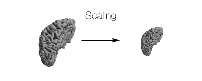
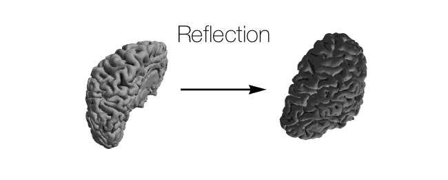
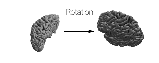
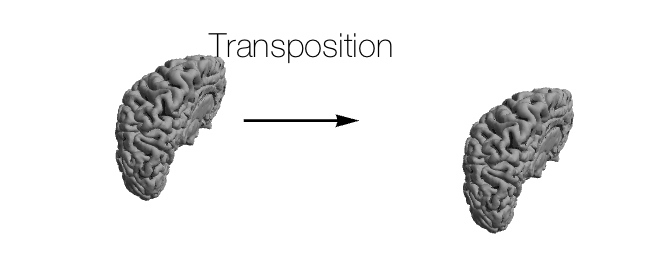
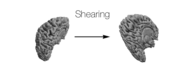
Other: \(f(\boldsymbol{v}) = \boldsymbol{0}\) is technically a linear transformation, but transformations not listed above don’t usually come up in neuroscience, and even shearing is very rarely used.

Usually, in neuroscience, the only transformations that matter are reflection, rotation, and translation; occasionally scaling comes into play as well. Of these four transformations, all but translation can be represented together in a \(3 \times 3\) matrix where:

\[\begin{pmatrix}x\\y\\z\end{pmatrix} = \begin{pmatrix}a & b & c\\d & e & f\\g & h & i\end{pmatrix} \cdot \begin{pmatrix}x_0\\y_0\\z_0\end{pmatrix}.\]

For more information about how matrices can act as linear transformations, see this page for a technical description and this page for more of a linear algebra review. This page is also decent for getting some intuition about the connection between the matrices and the transformations themselves.

Translation can be done by simply adding a 3D vector to this result. However, an alternate way to store translation along with the other transformations described above is to use a \(4 \times 4\) matrix, which is often called an affine transformation matrix. We write this transformation as:

\[\begin{pmatrix}x\\y\\z\\1\end{pmatrix} = \begin{pmatrix}a & b & c & t_x\\d & e & f & t_y\\g & h & i & t_z\\0 & 0 & 0 & 1\end{pmatrix} \cdot \begin{pmatrix}x_0\\y_0\\z_0\\1\end{pmatrix}.\]

Because they can succinctly store all of these transformations in a single matrix, affine transformation matrices are used in neuroscience volume files to tell the user how to align the data contained within them to some standard reference.

Orientations

(Back to Top)

In the example image (illustrating the radiological/neurological perspective conflict) above, it is clear that were the radiologist and the neurologist to design different file standards for an MRI volume file, they might prefer to organize the voxels in slightly different ways. The radiologist would probably want the slices of the image stored in the file starting with the bottom of the head (as slice 0) and ending with the top of the head; the neurologist may want the slices stored in a different order. In fact, there’s no particular right or wrong way to store the slices, and the slices needn’t even be horizontal slices. In some experiments the slices will be coronal or sagital. In order to efficiently express the ordering of the rows, columns, and slices of the file, a standard three-letter code can be used where each letter indicates the direction (Right/Left, Anterior/Posterior, Superior/Inferior) that is increasing for the particular dimension; for example, orientation SPL would indicate that the first dimension is pointing in the Superior direction, the second dimension is pointing in the Posterior direction, and the third dimension is pointing in the Left direction. WARNING: the convention I just described is used by FreeSurfer and other software but not all software. In particular, I believe that AFNI uses the opposite notation, where SPL would instead be represented as IAR; however, I do not use AFNI myself and unsure if this is (still) true. Check your favorite software’s documentation to be certain!

The most common orientations I see are:

RAS. The way we typically think about the position and coordinate system of our own brain is in a RAS orientation where the \(x\)-axis points out your right ear, the \(y\)-axis points out your nose, and the \(z\)-axis points out the top of your head. Surface files are almost always stored in a RAS coordinate system, and many other volume files are as well.
LIA. FreeSurfer uses LIA orientation for all of its volumetric data files. This means that the first dimension stored in the volume increases to the left, the next increases to the right, and the slices increase from posterior to anterior. I do not completely understand why this particular orientation was chosen by MGH. This website is very useful for understanding FreeSurfer’s volumetric coordinate system more fully.
LPS. The Winawer lab A/P slice prescription in various protocols (e.g., that used for retinotopy) yields LPS oriented volume files.

As a demonstration of what the orientation means in the context of the voxels and the 3D arrays that store them, consider the following Python code block. In it, we load a subject’s left hemisphere ribbon (the LH ribbon is a FreeSurfer volume file in which all the voxels in the LH gray matter are 1 and all other voxels are 0) and plot slices from it along each dimension. Because we know that the voxels are in the left hemisphere, it’s easy to tell which direction is which. In the example, I’ve labeled the axes in terms of their orientations. By plotting these data, we can see what it means, in terms of the 3D array representation, for a file to have an LIA orientation, which FreeSurfer uses by default.

import matplotlib.pyplot as plt
import neuropythy as ny

sub = ny.freesurfer_subject('bert')
vol = sub.lh_gray_mask

(f, (ax_xy, ax_yz, ax_xz)) = plt.subplots(1,3, figsize=(12,4))

ax_xy.imshow(vol[:,:,100].T,  cmap='gray', origin='lower')
ax_xy.set_xlabel('Index $i$ (R $\mapsto$ L)')
ax_xy.set_ylabel('Index $j$ (S $\mapsto$ I)')

ax_yz.imshow(vol[160,:,:].T, cmap='gray', origin='lower')
ax_yz.set_xlabel('Index $j$ (S $\mapsto$ I)')
ax_yz.set_ylabel('Index $k$ (P $\mapsto$ A)')

ax_xz.imshow(vol[:,100,:],   cmap='gray', origin='lower')
ax_xz.set_xlabel('Index $k$ (P $\mapsto$ A)')
ax_xz.set_ylabel('Index $i$ (R $\mapsto$ L)')

plt.tight_layout()

example_slices

Why does FreeSurfer use LIA orientation? Looking at these examples, it is clear that the LIA orientation does not make much sense when we plot the axes in a typically mathematically-oriented way (right-hand 3D coordinate system), as above. Neither is the LIA orientation quite the same as the radiological orientation shown in the cartoon above–though its \(x\)-coordinate is the same. I don’t know the answer to this question; though I suspect that whoever chose it wanted to view the first two dimensions (LI) as the \(x\) and \(-y\) axes of an image with increasing slices of the MR image coming out of the screen; this would give a RAS-like (right-handed) representation similar to the surface coordinates but where the brain is looking toward you as a viewer. Why \(x\) and \(-y\) are the obvious interpretations of the L and I directions in this case is not clear, however. It might be due to the fact that screens and images encode their \(y\) dimension (rows) from top-to-bottom; however when an array is drawn as an image, it’s first dimension (L in this case) is usually taken to be the rows of the image (\(-y\)) while its second dimension (I) is usually taken to be the columns of the image (\(x\)). Accordingly, it seems to me that ILA is at least as natural of a 3D-image orientation as LIA. The LIA orientation isn’t a choice I understand.

Relationship to Voxels and Volumes

(Back to Top)

NifTI and MGH files always contain at least one affine transformation matrix, as we saw in the examples above. The purpose of this transformation varies by file, however. In most cases, the matrix is used to tell the user how to align the voxels with some other reference. This reference might be a standard brain/space such as Talairach coordinates or MNI, or it might be the coordinate system for the surface representation of the brain.

Regardless of what the affine transformation aligns the voxels to, the coordinates being transformed are usually the 0-based indices of the voxels, which I will call \((i,j,k)\). So, for example, if \(\mathbf{M}\) is a \(4\times 4\) affine transformation matrix from the header of a volume file, then:

\(\begin{pmatrix}x\\y\\z\\1\end{pmatrix} = \mathbf{M} \cdot \begin{pmatrix}i\\j\\k\\1\end{pmatrix}\).

There is no single convention for what an affine transformation in a volume file actually means, so it is unwise to assume that you know the correct orientation of a file you obtained from someone else just because the affine transformation looks familiar. The NifTI file standard in fact includes two affine transforms, the “qform” and the “sform” with special numbers in the header that are supposed to give the user a hint as to what the transformations align the voxels to. Interpreting these values is beyond the scope of this post; I generally suggest keeping the qform and sform matrices identical in NifTI files to avoid confusion.

FreeSurfer. The affine transformation stored in most FreeSurfer mgh/mgz files in a subject’s directory (such as those shown in the examples above of brain.mgz) align the voxel indices with a RAS oriented space that I usually call “FreeSurfer native”; confusingly, this is not quite the same coordinate system as used in FreeSurfer’s surface files, though this latter transformation can be derived from the former. See the section on surface data below for details on how FreeSurfer’s various coordinate systems align.

Cortical Surfaces

(Back to Top)

The cortical surfaces is a 2D manifold embedded in a 3D space; accordingly, representing it in a computable format requires a bit more complexity than representing an MR image, which is just a 3D array. One cannot exactly represent the complex curvature of the cortex at every point due to the complexity of such a description and the limited resolution (usualy 0.8 mm\(^3\) at best) of our anatomical images of the brain. Instead, we must accept an approximate description of the cortical surface as described by a large set of small triangles, where all vertices lie on the surface itself.

When programs like FreeSurfer deduce the cortical surface from an anatomical MR image, they essentially make a good guess, based on the voxel intensities, of where a bunch of points/triangles lie on the boundary between white and gray (or gray and extra-cortical) matter. These points and triangles are then run through a variety of cleaning and smoothing routines to arrive at the representation of the white and pial surfaces. To see how these are made up of triangles and vertices, this image shows a zoomed in view of the pial surface as estimated by FreeSurfer.

surface_closeup

In addition to the added complexity of their data representations, surfaces also have fundamentally different storage needs when it comes to geometric data and other kinds of data such as parameter data. Recall that in a volume file, both the anatomical data and other data (such as model parameters or morphological data like curvature or thickness) can be stored in the voxels. On a surface, the anatomical information consists of vertices (a \(3\times n\) matrix of real numbers) and triangles (stored in a matrix of integers; see below) while the “property” data (parameters or morphological values) are stored in a vector of values (one for each vertex). Because of this, it is not convenient to store parameter values in the same kind of file as the anatomical values; therefore we need an understanding of how property and geometry files are related to each other.

Caveats

(Back to Top)

As of when this post was written, I do not feel that there is any single universally known or accepted surface file format for any kind of surface data. There are a variety of available formats used by various software (FreeSurfer, Caret/Workbench, for example), but one of the most common ways to store surface property data is still by encoding it in a NifTI or MGH volume file with size \(1\times 1 \times n\). For the most part, this isn’t too big of a deal because, relative to the clear possibilities of confusion with strangely-oriented volume files, surface files are relatively hard to confuse. It is rare that a subject will have the same number of vertices in their left and right hemispheres (in FreeSurfer at least), so even these are difficult to mix up. Nonetheless, it’s best to clearly communicate the format and conventions you are using whenever sharing surface files.

Geometry Data

(Back to Top)

Fortunately, he geometry of a cortical surface is virtually always stored in an ideomatic fashion, regardless of the file format. Although different formats may encode the data differently, these conventions are always present:

The vertices on the cortical surface are stored as an \(n\times 3\) matrix of real numbers. Warning: You should never assume that there is any rhyme or reason to the ordering of this matrix. Nearby vertices on the surface will not necessarily be nearby in this matrix.
The triangles of the cortical surface are sotred as an \(m\times 3\) matrix of non-negative integers where the integers are indices into the matrix of vertices, usually in a 0-based indexing system. I.e., if the first row of the matrix contained the integers \((1,4,88)\) that would indicate that the second, fifth, and eighty-ninth vertices were the corners of the first triangle on the cortical surface. Again, you should not assume any rhyme or reason to the ordering of the triangles in this matrix.
However, the columns of the triangle matrix will always list the vertices in a counter-clockwise direction with respect to an outward pointing surface normal vector. This is not generally important in a typical surface-based analysis, but it can be very important when calculating certain geometric data about a cortical surface.

FreeSurfer Files

(Back to Top)

FreeSurfer stores its surface data in a custom-format file type without a name or even an extension. You can find these files in any FreeSurfer subject’s /surf/ directory. The most important of these geometry files are:

lh.white and rh.white, the white surface representations for each hemisphere;
lh.pial and rh.pial, the pial surface representations;
lh.inflated and rh.inflated, inflated hemispheres appropriate for visualization;
lh.sphere and rh.sphere, a fully-inflated spherical version of each hemisphere;
lh.sphere.reg and rh.sphere.reg, the same spherical representation after anatomical alignment with the fsaverage subject (see surface alignment, below);
lh.fsaverage_sym.sphere.reg and ../xhemi/surf/lh.fsaverage_sym.sphere.reg, the same spherical representation registered to the fsaverage_sym left-right symmetric pseudo-hemisphere–this is generally only used for comparing left and right hemispheres.

Critically, all of these files for a single subject contain exactly the same set of triangles and all of them list their vertices in the same order. This means that each vertex is considered to have a position on the white surface, the pial surface, and the various inflated surfaces. Each triangle on the white or pial surface can therefore be thought of as a triangular prism that extends from the white to the pial surface as well.

The following code snippets demonstrate how to read these files.

Python (using nibabel)

import nibabel.freesurfer.io as fsio
  
(coords, faces) = fsio.read_geometry('/Volumes/server/Freesurfer_subjects/wl_subj042/surf/lh.white')

(type(coords), coords.shape, coords.dtype)
#=> (numpy.ndarray, (150676, 3), dtype('float64'))
  
(type(faces), faces.shape, faces.dtype)
#=> (numpy.ndarray, (301348, 3), dtype('>i4'))

Python (using neuropythy, which wraps nibabel)

import neuropythy as ny
  
sub = ny.freesurfer_subject('wl_subj042')

coords = sub.lh.white_surface.coordinates
faces  = sub.lh.tess.faces
# Note that ny.load() can also import freesurfer geometry files as surface meshes
  
(type(coords), coords.shape, coords.dtype)
#=> (numpy.ndarray, (3, 150676), dtype('float64'))

(type(faces), faces.shape, faces.dtype)
#=> (numpy.ndarray, (3, 301348), dtype('>i4'))

# (Note: neuropythy stores the coordinates and faces in a transposed form)

Matlab

addpath(genpath('/Applications/freesurfer/matlab')); % (FS installation dir on Mac)
  
[coords, faces] = read_surf('/Volumes/server/Freesurfer_subjects/wl_subj042/surf/lh.white');
  
size(coords)
%
% ans =
% 
%       150676           3
%

size(faces)
%
% ans =
% 
%       301348           3
%

Mathematica (using Neurotica)

<<Neurotica`
  
surf = Import[
  "/Volumes/server/Freesurfer_subjects/wl_subj042/surf/lh.white",
  "FreeSurferSurface"];
    
(* Alternately: *)
surf = Cortex[FreeSurferSubject["wl_subj042"], LH, "White"];
  
Dimensions@VertexCoordinates[surf]
(*=> {150676, 3} *)
  
Dimensions@FaceList[surf]
(*=> {301348, 3} *)

Other Files

(Back to Top)

In addition to FreeSurfer’s files, there are various other ways of storing surface data. Brainstorm, for example, stores these data in Matlab (.mat) files, but still stores it as a pair of vertex and triangle matrices. Additionally, the Caret/WorkBench software used and developed by the Human Connectome Project uses the GifTI file format. The GifTI format is large and complex and a full examination of it is beyond the scope of this post. GifTI files can store not only vertex and triangle data but also property data as well as a variety of other data, all in a single file. Accordingly, it can be very difficult to interpret a GifTI file even when its data has been correctly read and validated by a library such as Python’s nibabel.

The Neuropythy and Nibabel libraries in Python, the Neurotica library in Mathematica, and the workbench tools provided through the Human Connectome Project can all import GifTI files to some degree, but do not try very hard to interpret them for the user.

Property Data

(Back to Top)

Property data tends to take a few forms in FreeSurfer and other software; in FreeSurfer, these are label, annotation, and morphological (or ‘curv’) files. Label files are fairly simple, as they store either a mask of vertices in a particular ROI or a probability that each vertex is included in a particular ROI. Annotation and label files are beyond the scope if this post (I do not use them particularly often), but they are relatively straightforward to read with the libraries demo’ed in this post. For more information, see the documentation for nibabel.read_annotation, nibabel.read_label, and the help text for FreeSurfer’s read_label and read_annototation functions; additionally, the Neuropythy library can load these files with its ny.load() function, and the Neurotica library can adds importers for labels and annotations in Mathematica (named “FreeSurferLabel” and “FreeSurferAnnotation”).

Aside from annotation and label files, there are morphological or curv files, which can be used to store a single value on each vertex of the cortical surface. I consider this to be the most flexible method for storing surface data, as it can store labels and annotations as easily as anything. Because property data is just a list of vertices, however, it is also the case that typical volume files (MGH and NifTI format) can store surface property data. Such files will have two of their three first dimensions equal to one.

One relatively obvious convention is important for understanding how to map cortical surface property data onto the vertices in the cortical surface geometry files: the order of the vertices in the geometry’s coordinate matrix is the same as the ordering of the vertex properties in any of the property data files.

FreeSurfer Files

(Back to Top)

As mentioned above, FreeSurfer has its own custom format for storing surface properties. These files are usually called morphological or ‘curv’ files. Like FreeSurfer’s geometry files, these files have no extension; examples include lh.curv, lh.thickness, and rh.sulc, all of which live in a subject’s /surf/ directory.

FreeSurfer’s curv files contain a small amount of meta-data, but this almost never comes into play and isn’t discussed here. For most purposes, these files contain only a vector of values. The following code snippets demonstrate loading these data.

Python

# With nibabel...
import nibabel.freesurfer.io as fsio
  
dat = fsio.read_morph_data('/Volumes/server/Freesurfer_subjects/wl_subj042/surf/lh.curv')
dat.shape
#=> (150676,)
  
# With neuropythy...
import neuropythy as ny
dat = ny.freesurfer_subject('wl_subj042').lh.properties['curvature']
dat.shape
#=> (150676,)

Matlab

addpath(genpath('/Applications/freesurfer/matlab')); % (FS installation dir on Mac)
  
dat = read_curv('/Volumes/server/Freesurfer_subjects/wl_subj042/surf/lh.curv');
size(dat)
%
% ans =
% 
%       150676           1
%

Mathematica

<<Neurotica`
  
dat = Import[
  "/Volumes/server/Freesurfer_subjects/wl_subj042/surf/lh.curv",
  "FreeSurferCurv"];
Dimensions[dat]
(*=> {150676} *)
  
(* Or... *)
surf = Cortex[FreeSurferSubject["wl_subj042"], LH, "White"];
dat = "Curvature" /. surf;
Dimensions[dat]
(*=> {150676} *)

MGH and NifTI Files

(Back to Top)

Perhaps surprisingly, one of the most commonly used ways to store property data on the cortical surface that I’ve encountered is to put it in a 3D volume file where two of the 3 dimensions are unitary. When I do this, I try to ensure that the affine transform stored in the volume is the identity matrix in order to flag to any potential user that the header information is not relevant.

Note that in addition to storing a vector of scalars for each vertex in a 3D volume file, one can also store a set of vectors, one for each vertex, in such a file. This is difficult to do with other formats, so if, for example, you wish to store an interpolated time-series for each vertex or a 2D visual field coordinate for each vertex, you can do this by keeping only 1 unitary dimension in a 3D file; for example a time-series file for a cortical surface stored in a NifTI file might have the dimensions \((150\,676, 192, 1)\) where 150676 is the number of vertices in the surface and 192 is the number of time-points. When doing this, I suggest using the frames dimension (i.e., the fourth dimension) as the time-dimension as this is how it is typically represented in volumes. Additionally, if one writes a test in a script or function that checks if only one of the first three dimensions of a volume file is greater than 1, then such a test will still succeed (and, presumably, detect that the file contains surface-based data).

Importing surface data stored in a volume file can be done just as when importing a normal volume file. The only difference is that the neuropythy and Neurotica libraries both notice when a volume file contains only a vector or matrix, and, instead of returning 3D image objects, they return simple vectors or matrices.

Other Files

(Back to Top)

In addition to the file formats discussed above, GifTI files can store surface data but again are beyond the scope of this post. Really, once one understands that surface data is just a list of properties in an ordering that matches the vertex-ordering used in the appropriate geometry file, the file-format for these files becomes pretty uninteresting. Text files work pretty well for these data.

Alignments

(Back to Top)

Alignments in of MRI data in neuroscientific research take many forms. The most common of these is a simple rigid-body transformation (or affine transformation) such as that used to correct head-motion between frames of an EPI. Affine transformations are also needed to align volumes to cortical surfaces and vice versa. Surface-to-surface alignments usually refer to diffeomorphic alignments calculated in a 2D spherical geometric space (more on these below).

Volume-to-Volume

(Back to Top)

Although there exists software to perform diffeomorphic 3D alignments between brain volumes, these types of alignments are rare as of when this post was written and thus are not discussed in detail. For more information about such transformations, I recommend looking at ANTZ.

Most volume-to-volume transformations used in neuroscience are simple affine transformations represented by \(4\times 4\) matrices or a \(3\times 3\) matrix and a 3D translation vector. Such transformations are often generated for every frame of an fMRI time-series in order to align the images in the case of head motion. Note that if you have an affine transformation that aligns the voxels of file \(f\) with file \(g\), then the inverse matrix of the \(4\times 4\) affine transformation will align the voxels or vertices of of file \(g\) with the voxels of file \(f\).

Finding an Alignment Matrix

(Back to Top)

Finding an affine transformation that aligns one volume to another is usually the most difficult part of dealing with volume-to-volume alignments. The problem of finding a good alignment is not simple and won’t be discussed in this post. I will instead document a number of pieces of software of which I’m aware that can perform these computations.

FreeSurfer’s bbregister is probably the most common way to align volume data to/with a FreeSurfer subject. The bbregister program will align volumes such as EPIs to a subject’s anatomical images or to another EPI/BOLD image. The best documentation for bbregister can be found by running bbregister --help (or, better, bbregister --help | less). bbregister can either write out an alignment matrix in one of several formats or the aligned volume.
ITK-Snap is one of the better tools for aligning volumes by hand or refining alignments by hand. The user-interface for alignment is relatively easy to use. ITK-Snap saves out \(4\times 4\) affine alignment matrices in its own formats.
VistaSoft for Matlab can perform volumetric alignments; see this tutorial for more information.
Mathematica contains a large 3D image processing library and several image alignment algorithms that are potentially appropriate for MR images (see ImageAlign, FindGeometricTransform, ImageCorrespondingPoints, as well as this tutorial on image processing.

Volume-to-Surface and Surface-to-Volume

(Back to Top)

One almost never needs to actually find an affine transform that aligns a surface to a volume or vice versa; rather FreeSurfer has already found it (when it computed the surface in the first place), and one just reads it from a subject’s FreeSurfer directory (Caret/Workbench operate in a similar way; I am not familiar with AFNI, however). Finding an affine transformation between an arbitrary surface and a 3D anatomical volume is something that is certainly possible, but I do not know of any convenient software for performing this particular computation.

Rather, if you want to align subject A’s cortical surface with subject B’s anatomical volume, the best way to do this is to find the alignment matrix \(\mathbf{M}_{\mbox{A}_s \rightarrow \mbox{B}_v}\) that aligns subject A’sanatomical volume with subject B’s anatomical volume, then, combined with matrix \( \mathbf{M}_{\mbox{A}_s \rightarrow \mbox{A}_v}\) which aligns subject A’s cortical surface with their anatomical volume, calculate the desired alignment matrix \(\mathbf{M}_{\mbox{A}_s \rightarrow \mbox{B}_v}\):

\(\mathbf{M}_{\mbox{A}_s \rightarrow \mbox{B}_v} = \mathbf{M}_{\mbox{A}_v \rightarrow \mbox{B}_v} \cdot \mathbf{M}_{\mbox{A}_s \rightarrow \mbox{A}_v}\).

That said, determining the affine transformation matrix that aligns a FreeSurfer subject’s cortical surface with their cortical volume and vice versa is not trivial. Recall from earlier when we ran mri_info on a a FreeSurfer subject’s brain.mgz file (above). One of the pieces of information that this command printed about the file was an affine transformation matrix called the “voxel to ras transform” as well as its inverse, the “ras to voxel transform”. Because surfaces are almost always stored in a RAS configuration, one might expect that this affine transformation is the alignment of the volume file to the surface vertices. This, however, is incorrect. These alignment matrices align the volume with what I call “FreeSurfer native”. The FreeSurfer native coordinate system is identical to the vertex coordinate system except for a small translation that is different in every subject. In the subject bert above, the voxel-to-RAS alignment matrix was

\(\begin{pmatrix} -1 & 0 & 0 & 133.3997 \\ 0 & 0 & 1 & -110 \\ 0 & -1 & 0 & 128 \\ 0 & 0 & 0 & 1 \end{pmatrix}\).

Notice the translation coordinates in the first three rows of the last column. The voxel-to-vertex alignment matrix can be found by replacing these three values with \((128, -128, 128)\).

It is almost never necessary to create this voxel-to-vertex alignment matrix by hand; rather one can obtain them in a number of other ways. When one uses FreeSurfer tools to convert between FreeSurfer volumes and FreeSurfer surfaces, this special alignment is taken into account. The neuropythy library will also account for these differences automatically when performing interpolation (see below). The following code blocks demonstrate how to obtain the FreeSurfer surface-to-volume or volume-to-surface alignment matrix in a variety of languages.

Python (using nibabel)

import nibabel.freesurfer.mghformat as mgh
  
# MGH/MGZ files
mgh_file = mgh.load('/Volumes/server/Freesurfer_subjects/wl_subj042/mri/brain.mgz')
mgh_file.header.get_vox2ras_tkr()
#=> array([[  -1.,    0.,    0.,  128.],
#=>        [   0.,    0.,    1., -128.],
#=>        [   0.,   -1.,    0.,  128.],
#=>        [   0.,    0.,    0.,    1.]], dtype=float32)

Python (using neuropythy)

import neuropythy as ny
  
sub = ny.freesurfer_subject('wl_subj042')
sub.voxel_to_vertex_matrix
#=> array([[  -1.,    0.,    0.,  128.],
#=>        [   0.,    0.,    1., -128.],
#=>        [   0.,   -1.,    0.,  128.],
#=>        [   0.,    0.,    0.,    1.]], dtype=float32)

Matlab

addpath(genpath('/Applications/freesurfer/matlab')); % (FS installation dir on Mac)
  
mgh = MRIread('/Volumes/server/Freesurfer_subjects/wl_subj042/mri/brain.mgz');
mgh.tkrvox2ras
% 
% ans =
% 
%       -1.0000         0         0  128.0000
%             0         0    1.0000 -128.0000
%             0   -1.0000         0  128.0000
%             0         0         0    1.0000
% 

Surface-to-Surface

(Back to Top)

Surface-to-surface alignment is a much different beast than the previous two kinds of alignment. Surface-to-surface alignment usually involves a diffeomorphic mapping that brings the vertices in the inflated spherical surface representation of one subject into register with the spherical surface of another subject or atlas. When FreeSurfer processes an anatomical image, it automatically performs an alignment between the subject’s cortical surface and the atlas subject fsaverage. The fsaverage subject was constructed from the average brain of 40 subjects and thus has very smooth features. Alignment to the average brain is performed in FreeSurfer by minimizing the difference in the curvature and convexity (or sulcal depth) values (originally calculated on the white surface) between the vertices of the two subjects by warping the vertices of one. When FreeSurfer does this for your subject during recon-all, it creates the files lh.sphere.reg and rh.sphere.reg. These files still contain the same number of vertices and the same triangles as the subject’s other surface files, but the vertices are in slightly different positions relative to the lh.sphere and rh.sphere files. To align subjects in FreeSurfer, the surfreg command can be used. See this page for official documentation on it; though surfreg --help is probably more useful. Once a subject’s surface has been aligned with another subject’s or with an atlas, interpolation of the data from one sphere to the other should theoretically move the data between approximately equivalent anatomical structures; see surface-to-surface interpolation, below.

One important caveat to surface registrations and alignments involves a subject called fsaverage_sym. This subject, like fsaverage is an average atlas designed to be a target for alignment and group-average analysis. However, unlike the fsaverage, the fsaverage_sym is designed for alignments of both LH and RH cortices on the same hemisphere. In this sense, the fsaverage_sym is sometimes called a left-right symmetric pseudo-hemisphere. Data can be aligned to the fsaverage_sym subject by inverting the right hemisphere (using the xhemireg command or the --xhemi option to surfreg) and aligning it, along with the uninverted left hemisphere, to the fsaverage_sym subject’s left hemisphere. See this page for more information.

Interpolation

(Back to Top)

Transferring data from one format or coordinate system to another is almost always a process of alignment followed by interpolation. For example, to transfer data from a subject’s volume file to that subject’s surface, one first gets the affine transformation that aligns the subject’s surface vertices with the voxel’s indices, applies that transformation to the surface vertices, then performs interpolation (e.g., nearest-neighbor or tri-linear) on the vertex positions. This section discusses how interpolation is done, both from a high-level command-line perspective as well as in various programming languages.

From a Volume…

(Back to Top)

Suppose you have a volume file containing parameter data from a pRF model that you’ve solved for a subject. You want to get that data into another format–either a surface representation or another volume orientation. In this situation, the various data are usually called the target, the volume or vertices onto which you are interpolating, and the movable volume, the vertices from which you are interpolating. The solution to transferring this data is to follow the following steps:

Start with the target coordinates; for a surface target, these are the vertex coordinates, and for a volume target these are the voxel indices. Align these with the movable volume using whatever affine transform aligns the two. This yields the aligned coordinates.
For each aligned coordinate, calculate the interpolation within the voxels of the movable image. For nearest neighbor interpolation, this can be done by simply rounding the coordinate to the nearest integers.
The interpolated values at the original target coordinates form the data transferred between representations or coordinate systems.

Generally speaking, you won’t have to perform this operation manually, but it’s useful to know how it would work.

Nearest-Neighbor Interpolation

(Back to Top)

Volume-to-volume interpolation is generally performed as either a nearest-neighbor interpolation or as a trilinear interpolation. Nearest-neighbor interpolation simply assigns to each vertex index or voxel index from the target image the value of the voxel in the movable image that is closest to the aligned position of the indexed vertex or voxel. This is often a solid and simple choice when interpolating volumes, but can be problematic under certain conditions and is particularly prone to partial-voluming errors. See quandaries below.

Linear Interpolation

(Back to Top)

Linear interpolation is performed by assuming that there should be a smoothly-varying field between the voxel centers of a valume and that the second derivative of that field is 0. Linear interpolation of a point within a set of voxels is illustrated by the following diagram. Note that in the diagram, the dots represent the voxel centers of the 8 voxels nearest the point onto which one is interpolating.

trilinear_interpolation

In the diagram, the volume of the box is the weight assigned to the value at the voxel center with the same color. Notice that each box goes with the voxel-center farthest from it; this, however, gives a linear weighting between voxel centers that varies linearly. The weighted sub of values with the weights gives the resulting interpolated value.

Note that linear interpolation can use additional weights for each voxel as well, for example if you have a measure of the variance explained for a parameter estimation, you might want to use it as an additional weight when interpolating.

Heaviest-Neighbor Interpolation

(Back to Top)

Heaviest-neighbor interpolation is effectively just a weighted version of nearest-neighbor. The heaviest-neighbor interpolated value is calculated exactly as a linearly interpolated value except that instead of using a weighted sum of the neighboring values, the assigned interpolated value is that of the voxel whose weight is greatest. If no additional weights are given to a heaviest interpolation, then the result is identical to nearest-neighbor interpolation.

Tools and Examples

(Back to Top)

FreeSurfer’s mri_vol2vol and mri_vol2surf programs are one go-to solution for the problems described above. Both have somewhat steep learning curves as their documentation is sparse. For the best information on them, see mri_vol2vol --help and mri_vol2surf --help. Although mri_vol2vol tends to work fine in my experience, see FreeSurfer Quandaries below regarding mri_vol2surf.

Python, volume-to-surface (using neuropythy)

import neuropythy as ny
  
sub = ny.freesurfer_subject('wl_subj042')
img = sub.mgh_images['ribbon']
(lh_prop, rh_prop) = sub.image_to_cortex(img, method='nearest')
# Note: image_to_cortex supports 'linear' and 'heaviest' methods; additionally,
# options allow one to specify the surface onto which the interpolation is
# performed and to specify weights.
#
# image_to_cortex requires that the image include an affine transformation
# that aligns the voxels to the subjects 'FreeSurfer native' orientation
# (all of the subject's .mgz files contain this transformation).

[{k:np.sum(p == k) for k in np.unique(p) if k != 0} for p in [lh_prop,rh_prop]]
#=> [{2: 3597, 3: 126455, 41: 216}, {2: 313, 41: 3274, 42: 126917}]
# Note: a small number of incorrect-hemisphere values do wind up in the
# interpolated surface; this can't be helped when the vertices on the surface
# lie nearest to voxels in the opposite hemisphere.

From a Surface…

(Back to Top)

Interpolating from a surface is quite a bit tricker than interpolating from a volume, both conceptually and in terms of the algorithms required. For one, consider that, given a coordinate onto which to interpolate, it is not even clear if the coordinate is even on the surface. For that matter, it is not clear that a coordinate should have to be on the surface in order to be interpolated. Cortices are sheets, after all, and being between the white and pial surfaces should be sufficient to predict a value. For this precise reason, the neuropythy library treats interpolation of surfaces into volumes as a job for the Cortex object rather than a surface. This topic, which is highly relevant to interpolation of the ribbon from a surface representation, is discussed in the section on cortical sheets, below.

In the case of interpolating from surface to surface, i.e., from one subject to another or to the fsaverage atlas, interpolation should be done on the inflated spherical surface of the appropriate hemispheres. Using the spherical surfaces actually solves one of the problems mentioned above because every vertex on one sphere must be inside of a triangle of the other sphere, unless the spheres have holes somewhere. The spherical surfaces used in these interpolations should be aligned by FreeSurfer before use.

Assuming that one has an aligned pair of spherical surfaces, then the concept of nearest-neighbor interpolation between voxels is quite trivial. Linear interpolation within a triangle is also similar in concept to the trilinear interpolation used in voxels (above). The following diagram shows the triangular equivalent. See also barycentric coordinates.

triangle_linear_interp

Heaviest-neighbor interpolation in surfaces is essentially identical to the method used in volumes as well..

Tools and Examples

FreeSurfer’s mri_surf2surf is a good way to perform surface-to-surface interpolation, but it is poorly documented and somewhat complex. The best documentation is probably found via mri_surf2surf --help. On the other hand, FreeSurfer’s mri_surf2vol has fairly spotty results, at least prior to FreeSurfer version 6; see quandries below.

Python, surface to volume (using neuropythy)

import neuropythy as ny
  
sub = ny.freesurfer_subject('wl_subj042')
img = sub.cortex_to_image((sub.lh.prop('curvature'), sub.rh.prop('curvature')),
                          method='linear', dtype='float')
# Note: cortex_to_image supports 'nearest' and 'heaviest' methods
plt.imshow(img[:,100,:], cmap='gray')

neuropythy_curv_surf2vol

Python, surface to surface (using neuropythy)

import neuropythy as ny
  
sub = ny.freesurfer_subject('wl_subj042')
fsa = ny.freesurfer_subject('fsaverage')
curv_on_fsa = fsa.lh.interpolate(sub.lh.prop('curvature'), method='linear')
# Note: the interpolate function automatically detects when the two subejcts
# are registered to each other and uses that registration.

Common Quandaries

(Back to Top)

The following are caveats and quandaries that come up in practice when dealing with the kind of data and transformations described on this page, particularly interpolation.

FreeSurfer’s Interpolation Tools

(Back to Top)

FreeSurfer includes a number of useful utilities, most of which are excellent. I have, however, noticed issues with the mri_vol2surf and mri_surf2vol programs on occasion. Specifically, the results of these interpolations are frequently quite spotty or inaccurate; sometimes they do not appear to fill the ribbon or they assign a value to every vertex on the cortical surface. It is possible that newer versions of these programs that I have not used have fixed these issues (note: I have not tested FreeSurfer 6 as of writing this post), but I don’t currently recommend that people use these when there are other options available.

Cortices as Sheets

(Back to Top)

The pial and white cortical surfaces are clearly surfaces, but the cortex itself is a sheet with volume, not a 2D manifold. The voxels of the ribbon, should be between the white and pial surfaces, and accordingly, should be assigned values not based on their nearest vertex neighbor but based on their position inside of the triangular prism that contains them. Both heaviest and linear interpolation methods should, in theory, take into account this geometry when performing interpolation.

To my knowledge, the only library or tool that performs interpolation from vertex-to-voxel is the neuropythy library. This is done in neuropythy by using a generalization of barycentric coordinates to tetrahedrons, which are drawn between the pial and white surfaces. The library even allows you to specify different values for the white and pial surfaces, giving different layers of the ribbon to assume different values.

Written on January 26, 2018

Noah C. Benson

MRI Data Representation and Geometry

Table of Contents

Introduction

File Formats

Cortical Volumes (EPIs and Anatomical Images)

Voxel Data

Meta-Data

Accessing Meta-Data

MRImage Geometry

Affine Transformations

Orientations

Relationship to Voxels and Volumes

Cortical Surfaces

Caveats

Geometry Data

FreeSurfer Files

Other Files

Property Data

FreeSurfer Files

MGH and NifTI Files

Other Files

Alignments

Volume-to-Volume

Finding an Alignment Matrix

Volume-to-Surface and Surface-to-Volume

Surface-to-Surface

Interpolation

From a Volume…

Nearest-Neighbor Interpolation

Linear Interpolation

Heaviest-Neighbor Interpolation

Tools and Examples

From a Surface…

Tools and Examples

Common Quandaries

FreeSurfer’s Interpolation Tools

Cortices as Sheets