k-Means Clustering

Clustering is one of the most common and useful tools in the data scientists arsenal. Frequently, real world problems revolve around the ability to recognize what “class” of thing something is based on some measurements of it. For example, the ability to identify a chemical from its spectral readings is fundamentally a classification problem. Clustering is a kind of approach to classification based on similarity between data points.

The k-means clustering algorithm is one of the most intuitive unsupervised learning algorithm. It’s goal is to deduce natural clusters in a dataset by figuring out which data points are most similar to each other. It’s called “k-means” because it results in \(k\) classes using a method that attempts to find the mean of each class of data points.

How k-Means Clustering Works

Many machine learning methods work via a similar pattern: (1) they make a guess about the answer, (2) they make a small change to the guess that improves its goodness slightly, then (3) they repeat step 2 until the guess is “good enough” in some way. The k-means algorithm is a great example of this approach. It works as follows.

K-Means Algorithm

Inputs

1. A set of points. There may be any number of points, and they may have any number of dimensions (columns). All the dimensions should be numerical.

2. \(k\). The number of clusters to find.

Algorithm

1. Guess. The algorithm randomly chooses \(k\) points. These “cluster points” will have the same dimensionality as the input points.

2. Iterate. These steps are performed repeatedly until some threshold is reached.

   1. Assign clusters. For each point in the input, the algorithm figures out which of the \(k\) cluster points is closest to it and assigns it that cluster value.

   2. Update clusters. For each cluster, update the position of the cluster point to be the mean of all input points that belong to the cluster.

Outputs

1. The \(k\) cluster points representing the \(k\) clusters found by the method; each data point is the mean position of all the data points in one of the \(k\) clusters.

2. An assignment of all the input points into one of the \(k\) clusters.

Demonstration

The following animation demonstrates how the k-means algorithm works generally.

In this animation, the black dots are the data points that we are hoping to cluster based on their (x,y) position. Each star represents one of the three clusters.

Initially, the three stars have a random position that doesn’t do a very good job of representing where the underlying clusters are. However, after a few iterations of the k-means algorithm, in which we repeatedly assign each data point to its nearest cluster then move each cluster’s position to the mean position of its assigned data points, we reach a good clustering.

Once Loop Reflect

Example: Finding Clusters in the California Housing Dataset

Let’s work through an example of k-means clustering with a real dataset. We’ll use the California Housing Dataset that we examined earlier in the Introduction to Unsupervised Learning, and we’ll attempt to find geographical clusters of census parcels using k-means clustering.

Load the Dataset

# First, we need to import scikit-learn:
import sklearn as skl

# Next, we use scikit-learn to download and return the CA housing dataset:
ca_housing_dataset = skl.datasets.fetch_california_housing()

# Extract the actual data rows and the feature names:
ca_housing_data = ca_housing_dataset['data']
ca_housing_featnames = ca_housing_dataset['feature_names']

# We also extract the target data:
ca_housing_targdata = ca_housing_dataset['target']
ca_housing_targnames = ca_housing_dataset['target_names']

# To organize the dataset into a dataframe, we use Pandas:
import pandas as pd

feat_df = pd.DataFrame(
    {k: v for (k,v) in zip(ca_housing_featnames, ca_housing_data.T)})
targ_df = pd.DataFrame({ca_housing_targnames[0]: ca_housing_targdata})

# Display the feature dataframe:
feat_df

	MedInc	HouseAge	AveRooms	AveBedrms	Population	AveOccup	Latitude	Longitude
0	8.3252	41.0	6.984127	1.023810	322.0	2.555556	37.88	-122.23
1	8.3014	21.0	6.238137	0.971880	2401.0	2.109842	37.86	-122.22
2	7.2574	52.0	8.288136	1.073446	496.0	2.802260	37.85	-122.24
3	5.6431	52.0	5.817352	1.073059	558.0	2.547945	37.85	-122.25
4	3.8462	52.0	6.281853	1.081081	565.0	2.181467	37.85	-122.25
...	...	...	...	...	...	...	...	...
20635	1.5603	25.0	5.045455	1.133333	845.0	2.560606	39.48	-121.09
20636	2.5568	18.0	6.114035	1.315789	356.0	3.122807	39.49	-121.21
20637	1.7000	17.0	5.205543	1.120092	1007.0	2.325635	39.43	-121.22
20638	1.8672	18.0	5.329513	1.171920	741.0	2.123209	39.43	-121.32
20639	2.3886	16.0	5.254717	1.162264	1387.0	2.616981	39.37	-121.24

20640 rows × 8 columns

Visualize the Longitude and Latitude Data

We can start by visualizing the raw data that we’re going to use for clustering. We’re using the longitude and latitude of each census parcel in the dataset, so a visualization of these coordinates should be resemble the state of California.

# Extract the longitude and latitude from the dataset features.
x = feat_df['Longitude']
y = feat_df['Latitude']

# We'll need matplotlib to make the plots:
import matplotlib.pyplot as plt
# Make a quick scatter-plot where each dot is a parcel center.
plt.scatter(x, y, c='k', s=0.5)
plt.xlabel('Longitude')
plt.ylabel('Latitude')
# Make sure the plot axis represents x and y space equally.
plt.axis('equal')
# Show the plot.
plt.show()

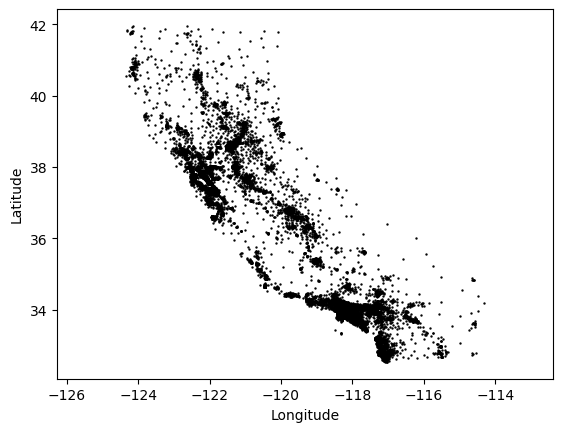
Clearly there are clusters of parcels near the most populated parts of the state: Los Angeles, San Diego, San Francisco and the Bay Area, and Sacramento in particular. While there is no one correct way to cluster the parcels in this map, we might assess that a method of clustering performs well if it tends to identify these areas as distinct clusters.

Let’s see how to use k-means for this task and how well it performs.

import numpy as np

# Make an (Nx2) coordinate matrix of the latitude and longitude:
coords = np.c_[x,y]
# Use scikit-learn's KMeans algorithm; we'll search for 8 clusters:
n_clusters = 8
kmeans = skl.cluster.KMeans(n_clusters=n_clusters)
kmeans.fit(coords)

Show code cell output

Hide code cell output

KMeans()

In a Jupyter environment, please rerun this cell to show the HTML representation or trust the notebook.
On GitHub, the HTML representation is unable to render, please try loading this page with nbviewer.org.

Once the above cell has been run, the kmean object has been fitted, meaning that it has found cluster centers and cluster labels for the parcels in the census. We can access these discovered values as fields of the kmeans object itself.

In scikit-learn, this paradigm is very common: one creates an object (i.e., a sklearn.cluster.KMeans object) that takes some parameters (the number of clusters), then you provide the object with data via a fit function. After calling the fitting routine, the object has been trained and its methods and fields can be queried.

The fields that scikit-learn provides for the user typically end with an underscore (_) character.

# This gives us one label per parcel in the census.
label = kmeans.labels_
# And one cluster center per cluster.
centers = kmeans.cluster_centers_

# Make another scatter plot of the parcels, but color them by their cluster
# label this time:
plt.scatter(x, y, c=label, s=0.5, cmap='hsv')
# Also plot the cluster centers as stars.
plt.scatter(
    centers[:,0], centers[:,1],
    edgecolor='k',
    c=np.linspace(0,1,n_clusters),
    cmap='hsv', 
    s=50,
    marker='*')
# Fix up the plot to use isomorphic pixel sizes.
plt.axis('equal')
# And plot the figure.
plt.show()

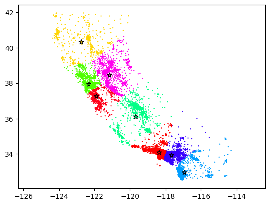
Clearly, the algorithm found some clusters that make sense, but it’s simultaneously hard to say whether these clusters are “correct” in any meaningful sense. In part, this is because geographic clustering is a complicated topic—politics, culture, geography, and population all play major roles in our societal notion of a geographical regions. However, k-means is also limited in that it cares only about a simple metric of closeness, and it’s simply not always the case that spatial closeness is a good indicator of whether two locations are part of a geographical cluster.

Note additionally that k-means is a stochastic algorithm, meaning that if you run it several times, you will likely get slightly different results each time. If you run the two cells above several times, you can get a sense for the kinds of clusterings k-means can produce from similar data.

After running the cell above several times, what are some of the strengths and weaknesses of this method that you observe?

Some possible strengths…

• K-means runs quickly. In fact, you can run it many times even for fairly large datasets.

• K-means classifies all points. There is never an outlier point that the k-means algorithm misses or fails to classify.

• K-means is easy to understand. The k-means method itself is straightforward, and others will have little trouble understanding results based on k-means.

Some possible weaknesses…

• K-means is not especially reliable. The answer you get differs quite a bit across different runs of k-means, at least for this problem.

• K-means can’t figure out the number of clusters. Often we won’t know the correct number of clusters and would rather the algorithm figure it out for us.

• K-means does not care about density. It does not try to draw cluster boundaries where the density is lowest.

Additional Resources

• k-means at Wikipedia

• k-means user-guide at Scikit-learn

• k-means documentation at Scikit-learn