Introduction to Neural Networks#
Neural Networks are flexible and powerful tools for learning that loosely model the neurons of the human brain. In the brain, neurons receive discrete signals from afferent neurons and accumulate them leakily over time. Once a certain threshold of signal is accumulated the neuron fires to its efferent neurons. Artificial neural networks (ANNs) work somewhat differently in that they are not sensitive to the timing of inputs in the same way—inputs flow from one layer of the ANN to the next as stages of the computation, but not as a simulation of time. However, artificial neurons do accumulate input from afferent neurons and send an accumulation of that input to efferent neurons.
In this section we’ll discuss the basic structure of neural networks. In the next section, we’ll discuss and work through examples of simple linear neural networks, followed by convolutional neural networks. In the final section, we’ll discuss some of the prebuilt ANNs that can be loaded using PyTorch.
What is an Artificial Neuron?#
Like real biological neurons, artificial neurons are computational units that collect information from input neurons and pass some summary of that information along to a set of output neurons. The input information in an ANN is weighted linearly, meaning that the when an ANN receives input from its afferent neurons, it multiplies each afferent’s input by a weight then calculates a weighted sum of the inputs. In a purely linear ANN, this sum is the neuron’s output. In nonlinear neurons, this sum is passed through an activation function, such as a sigmoid function or a simple threshold.
Note
The sigmoid function is sometimes used as an output function for neurons because it converts real numbers into probabilities. That is sigmoid(x) for any real-valued x will yield a real number between 0 and 1.
It is generally easier for neurons and neural networks to learn to predict very large numbers when, for example, their inputs match a category they recognize and very small numbers when their input doesn’t than it is to train them to predict a precise probability that their input is a member of their recognized category. Training ANNs to predict either large or small numbers then running those numbers through a sigmoid function at the end is a useful trick when one is predicting classes or probabilities with an ANN.
A little but more formally, the \(j\)th neuron of an ANN is defined by a few things:
The set of neurons from which it receives inputs. We call its inputs \(x_1\), \(x_2\) … \(x_n\) (\(n\) is the number of inputs to the neuron).
The weight on each input, \(w_1\), \(w_2\) … \(w_n\). Critically, these weights are the parameters of the model that are learned during training.
The transfer function, which accumulates the inputs. For our cases, this will always be \(w_1\,x_1 + w_2\,x_2 + ... + w_n\,x_n\).
The activation function \(\phi(y)\) which may be a sigmoid or a threshold. A threshold is essentially a function equivalent to
1 if y > theta else 0for some threshold valuetheta.

Image credit: Funcs, CC0, via Wikimedia Commons
What is an Artificial Neural Network?#
An Artificial Neural Network (ANN) is a collection of artificial neurons, usually organized into multiple layers. The first layer is called the “input layer”, the final layer is called the “output layer”, and the layers between which represent the computations are called “hidden layers”. Typically, the outputs of one layer form the inputs to the next layer, with each neuron in any particular layer receiving inputs from all neurons in the previous layer and providing outputs to all neurons on the following layer. The following diagram, in which each arrow represents a weighted input, and each circle represents an individual artificial neuron, illustrates this.

In the above diagram, the input consists of 4 values while the output consists of 1 value. Each arrow represents a unique weight. If the artificial neurons performed weighted summation only—i.e., without any activation function, then it should be clear that the layers are simply performing the multiplication of a weight matrix times an input vector. In other words, without an activation function to create some kind of nonlinearity, ANNs compute only linear operators.
Linear operators are quite useful, as we saw in Lesson 2.1, but linear regression is a far better way to train a linear operator than ANNs. Accordingly, most ANNs include some components that perform nonlinear activations. The most common of these activations are the following:
Sigmoid Function. The sigmoid function is defined as \(\sigma(x) = \frac{1}{1 + \exp(-x)}\). The function itself looks a bit like an S. It’s minimum value approaches 0 as \(x\) goes to \(-\infty\), and its maximum value approaches 1 as \(x\) goes to \(\infty\), so it can be understood as a transformation between real numbers and probabilities (\(\sigma(0) = 1/2\)). Sigmoid functions are often applied to ANN outputs to convert their internal representations into probabilities of membership in a class.
Threshold Function. The threshold funciton is defined for some threshold value \(\theta\) to be \(\phi(x) = 1 \mbox{ if } x > \theta \mbox{, otherwise } \phi(x) = 0\).
Rectified Linear Unit. Often abbreviated ReLU, the rectified linear unit is defined as \(r(x) = \max\{0, x\}\). ReLUs are very simple and very common in convolutional neural networks.
Different activation layers have different consequences for a neural network’s computations and its ability to model various kinds of problems, but understanding precisely what effects they have and how they change the model’s capabilities is beyond the scope of this course. One way to understand them, however, is as junctions in the computation performed by the ANN that allow the computation to make decisions (like if statements in Python). Without such junctions, there is just a linear equation. With the junctions, those linear equations can implement complex decisions.
The MNIST Dataset#
In the tutorials in this section, we’ll be using the MNIST dataset, which contains images of handwritten numerals (0-9), each of which has been labeled. We can load it in using the torchvision library, which is a companion library for PyTorch that specifically supports a variety of computer vision related tasks. The torchvision library isn’t required to use PyTorch effectively, but it contains a lot of handy utilities. More information can be found here.
Let’s use torchvision to load in the MNIST dataset and look at some exaples now.
from torchvision.datasets import MNIST
from pathlib import Path

# This will download the MNIST directory into your home directory.
# If you are using the docker image, the downloaded files will only exist
# inside the container.
train_dset = MNIST(Path.home(), download=True, train=True)
test_dset = MNIST(Path.home(), download=True, train=False)
The datasets themselves are already PyTorch Dataset objects, so they can be queried just like the dataset we created in the previous lesson.
# How many samples are in the training and test datasets?
print("Training samples:", len(train_dset))
print("Test samples:", len(test_dset))
Training samples: 60000
Test samples: 10000
# Extract a specific sample:
(sample_in, sample_out) = train_dset[0]

print("Input type:", type(sample_in))
print("Output type:", type(sample_out))
Input type: <class 'PIL.Image.Image'>
Output type: <class 'int'>
Notice that while the type of the sample outputs are int, which we expect given that each image represents a digit 0–9, but the input type is PIL.Image.Image. PIL stands for the Python Image Library, which contains utilities for reading and saving many image formats. A PIL Image object can represent an RGB or grayscale image—the latter in this case.
There are a number of ways to convert an image into a tensor, but there’s a simple utility that is included in torchvision that can do this for us called ToTensor. ToTensor is a type that’s actually meant to be used as a layer in a PyTorch Module. (Usually it’s the first layer, designed to make sure the input is a valid PyTorch tensor).
from torchvision.transforms import ToTensor

tt = ToTensor()
tens = tt(sample_in)
tens
tensor([[[0.0000, 0.0000, 0.0000, 0.0000, 0.0000, 0.0000, 0.0000, 0.0000,
          0.0000, 0.0000, 0.0000, 0.0000, 0.0000, 0.0000, 0.0000, 0.0000,
          0.0000, 0.0000, 0.0000, 0.0000, 0.0000, 0.0000, 0.0000, 0.0000,
          0.0000, 0.0000, 0.0000, 0.0000],
         [0.0000, 0.0000, 0.0000, 0.0000, 0.0000, 0.0000, 0.0000, 0.0000,
          0.0000, 0.0000, 0.0000, 0.0000, 0.0000, 0.0000, 0.0000, 0.0000,
          0.0000, 0.0000, 0.0000, 0.0000, 0.0000, 0.0000, 0.0000, 0.0000,
          0.0000, 0.0000, 0.0000, 0.0000],
         [0.0000, 0.0000, 0.0000, 0.0000, 0.0000, 0.0000, 0.0000, 0.0000,
          0.0000, 0.0000, 0.0000, 0.0000, 0.0000, 0.0000, 0.0000, 0.0000,
          0.0000, 0.0000, 0.0000, 0.0000, 0.0000, 0.0000, 0.0000, 0.0000,
          0.0000, 0.0000, 0.0000, 0.0000],
         [0.0000, 0.0000, 0.0000, 0.0000, 0.0000, 0.0000, 0.0000, 0.0000,
          0.0000, 0.0000, 0.0000, 0.0000, 0.0000, 0.0000, 0.0000, 0.0000,
          0.0000, 0.0000, 0.0000, 0.0000, 0.0000, 0.0000, 0.0000, 0.0000,
          0.0000, 0.0000, 0.0000, 0.0000],
         [0.0000, 0.0000, 0.0000, 0.0000, 0.0000, 0.0000, 0.0000, 0.0000,
          0.0000, 0.0000, 0.0000, 0.0000, 0.0000, 0.0000, 0.0000, 0.0000,
          0.0000, 0.0000, 0.0000, 0.0000, 0.0000, 0.0000, 0.0000, 0.0000,
          0.0000, 0.0000, 0.0000, 0.0000],
         [0.0000, 0.0000, 0.0000, 0.0000, 0.0000, 0.0000, 0.0000, 0.0000,
          0.0000, 0.0000, 0.0000, 0.0000, 0.0118, 0.0706, 0.0706, 0.0706,
          0.4941, 0.5333, 0.6863, 0.1020, 0.6510, 1.0000, 0.9686, 0.4980,
          0.0000, 0.0000, 0.0000, 0.0000],
         [0.0000, 0.0000, 0.0000, 0.0000, 0.0000, 0.0000, 0.0000, 0.0000,
          0.1176, 0.1412, 0.3686, 0.6039, 0.6667, 0.9922, 0.9922, 0.9922,
          0.9922, 0.9922, 0.8824, 0.6745, 0.9922, 0.9490, 0.7647, 0.2510,
          0.0000, 0.0000, 0.0000, 0.0000],
         [0.0000, 0.0000, 0.0000, 0.0000, 0.0000, 0.0000, 0.0000, 0.1922,
          0.9333, 0.9922, 0.9922, 0.9922, 0.9922, 0.9922, 0.9922, 0.9922,
          0.9922, 0.9843, 0.3647, 0.3216, 0.3216, 0.2196, 0.1529, 0.0000,
          0.0000, 0.0000, 0.0000, 0.0000],
         [0.0000, 0.0000, 0.0000, 0.0000, 0.0000, 0.0000, 0.0000, 0.0706,
          0.8588, 0.9922, 0.9922, 0.9922, 0.9922, 0.9922, 0.7765, 0.7137,
          0.9686, 0.9451, 0.0000, 0.0000, 0.0000, 0.0000, 0.0000, 0.0000,
          0.0000, 0.0000, 0.0000, 0.0000],
         [0.0000, 0.0000, 0.0000, 0.0000, 0.0000, 0.0000, 0.0000, 0.0000,
          0.3137, 0.6118, 0.4196, 0.9922, 0.9922, 0.8039, 0.0431, 0.0000,
          0.1686, 0.6039, 0.0000, 0.0000, 0.0000, 0.0000, 0.0000, 0.0000,
          0.0000, 0.0000, 0.0000, 0.0000],
         [0.0000, 0.0000, 0.0000, 0.0000, 0.0000, 0.0000, 0.0000, 0.0000,
          0.0000, 0.0549, 0.0039, 0.6039, 0.9922, 0.3529, 0.0000, 0.0000,
          0.0000, 0.0000, 0.0000, 0.0000, 0.0000, 0.0000, 0.0000, 0.0000,
          0.0000, 0.0000, 0.0000, 0.0000],
         [0.0000, 0.0000, 0.0000, 0.0000, 0.0000, 0.0000, 0.0000, 0.0000,
          0.0000, 0.0000, 0.0000, 0.5451, 0.9922, 0.7451, 0.0078, 0.0000,
          0.0000, 0.0000, 0.0000, 0.0000, 0.0000, 0.0000, 0.0000, 0.0000,
          0.0000, 0.0000, 0.0000, 0.0000],
         [0.0000, 0.0000, 0.0000, 0.0000, 0.0000, 0.0000, 0.0000, 0.0000,
          0.0000, 0.0000, 0.0000, 0.0431, 0.7451, 0.9922, 0.2745, 0.0000,
          0.0000, 0.0000, 0.0000, 0.0000, 0.0000, 0.0000, 0.0000, 0.0000,
          0.0000, 0.0000, 0.0000, 0.0000],
         [0.0000, 0.0000, 0.0000, 0.0000, 0.0000, 0.0000, 0.0000, 0.0000,
          0.0000, 0.0000, 0.0000, 0.0000, 0.1373, 0.9451, 0.8824, 0.6275,
          0.4235, 0.0039, 0.0000, 0.0000, 0.0000, 0.0000, 0.0000, 0.0000,
          0.0000, 0.0000, 0.0000, 0.0000],
         [0.0000, 0.0000, 0.0000, 0.0000, 0.0000, 0.0000, 0.0000, 0.0000,
          0.0000, 0.0000, 0.0000, 0.0000, 0.0000, 0.3176, 0.9412, 0.9922,
          0.9922, 0.4667, 0.0980, 0.0000, 0.0000, 0.0000, 0.0000, 0.0000,
          0.0000, 0.0000, 0.0000, 0.0000],
         [0.0000, 0.0000, 0.0000, 0.0000, 0.0000, 0.0000, 0.0000, 0.0000,
          0.0000, 0.0000, 0.0000, 0.0000, 0.0000, 0.0000, 0.1765, 0.7294,
          0.9922, 0.9922, 0.5882, 0.1059, 0.0000, 0.0000, 0.0000, 0.0000,
          0.0000, 0.0000, 0.0000, 0.0000],
         [0.0000, 0.0000, 0.0000, 0.0000, 0.0000, 0.0000, 0.0000, 0.0000,
          0.0000, 0.0000, 0.0000, 0.0000, 0.0000, 0.0000, 0.0000, 0.0627,
          0.3647, 0.9882, 0.9922, 0.7333, 0.0000, 0.0000, 0.0000, 0.0000,
          0.0000, 0.0000, 0.0000, 0.0000],
         [0.0000, 0.0000, 0.0000, 0.0000, 0.0000, 0.0000, 0.0000, 0.0000,
          0.0000, 0.0000, 0.0000, 0.0000, 0.0000, 0.0000, 0.0000, 0.0000,
          0.0000, 0.9765, 0.9922, 0.9765, 0.2510, 0.0000, 0.0000, 0.0000,
          0.0000, 0.0000, 0.0000, 0.0000],
         [0.0000, 0.0000, 0.0000, 0.0000, 0.0000, 0.0000, 0.0000, 0.0000,
          0.0000, 0.0000, 0.0000, 0.0000, 0.0000, 0.0000, 0.1804, 0.5098,
          0.7176, 0.9922, 0.9922, 0.8118, 0.0078, 0.0000, 0.0000, 0.0000,
          0.0000, 0.0000, 0.0000, 0.0000],
         [0.0000, 0.0000, 0.0000, 0.0000, 0.0000, 0.0000, 0.0000, 0.0000,
          0.0000, 0.0000, 0.0000, 0.0000, 0.1529, 0.5804, 0.8980, 0.9922,
          0.9922, 0.9922, 0.9804, 0.7137, 0.0000, 0.0000, 0.0000, 0.0000,
          0.0000, 0.0000, 0.0000, 0.0000],
         [0.0000, 0.0000, 0.0000, 0.0000, 0.0000, 0.0000, 0.0000, 0.0000,
          0.0000, 0.0000, 0.0941, 0.4471, 0.8667, 0.9922, 0.9922, 0.9922,
          0.9922, 0.7882, 0.3059, 0.0000, 0.0000, 0.0000, 0.0000, 0.0000,
          0.0000, 0.0000, 0.0000, 0.0000],
         [0.0000, 0.0000, 0.0000, 0.0000, 0.0000, 0.0000, 0.0000, 0.0000,
          0.0902, 0.2588, 0.8353, 0.9922, 0.9922, 0.9922, 0.9922, 0.7765,
          0.3176, 0.0078, 0.0000, 0.0000, 0.0000, 0.0000, 0.0000, 0.0000,
          0.0000, 0.0000, 0.0000, 0.0000],
         [0.0000, 0.0000, 0.0000, 0.0000, 0.0000, 0.0000, 0.0706, 0.6706,
          0.8588, 0.9922, 0.9922, 0.9922, 0.9922, 0.7647, 0.3137, 0.0353,
          0.0000, 0.0000, 0.0000, 0.0000, 0.0000, 0.0000, 0.0000, 0.0000,
          0.0000, 0.0000, 0.0000, 0.0000],
         [0.0000, 0.0000, 0.0000, 0.0000, 0.2157, 0.6745, 0.8863, 0.9922,
          0.9922, 0.9922, 0.9922, 0.9569, 0.5216, 0.0431, 0.0000, 0.0000,
          0.0000, 0.0000, 0.0000, 0.0000, 0.0000, 0.0000, 0.0000, 0.0000,
          0.0000, 0.0000, 0.0000, 0.0000],
         [0.0000, 0.0000, 0.0000, 0.0000, 0.5333, 0.9922, 0.9922, 0.9922,
          0.8314, 0.5294, 0.5176, 0.0627, 0.0000, 0.0000, 0.0000, 0.0000,
          0.0000, 0.0000, 0.0000, 0.0000, 0.0000, 0.0000, 0.0000, 0.0000,
          0.0000, 0.0000, 0.0000, 0.0000],
         [0.0000, 0.0000, 0.0000, 0.0000, 0.0000, 0.0000, 0.0000, 0.0000,
          0.0000, 0.0000, 0.0000, 0.0000, 0.0000, 0.0000, 0.0000, 0.0000,
          0.0000, 0.0000, 0.0000, 0.0000, 0.0000, 0.0000, 0.0000, 0.0000,
          0.0000, 0.0000, 0.0000, 0.0000],
         [0.0000, 0.0000, 0.0000, 0.0000, 0.0000, 0.0000, 0.0000, 0.0000,
          0.0000, 0.0000, 0.0000, 0.0000, 0.0000, 0.0000, 0.0000, 0.0000,
          0.0000, 0.0000, 0.0000, 0.0000, 0.0000, 0.0000, 0.0000, 0.0000,
          0.0000, 0.0000, 0.0000, 0.0000],
         [0.0000, 0.0000, 0.0000, 0.0000, 0.0000, 0.0000, 0.0000, 0.0000,
          0.0000, 0.0000, 0.0000, 0.0000, 0.0000, 0.0000, 0.0000, 0.0000,
          0.0000, 0.0000, 0.0000, 0.0000, 0.0000, 0.0000, 0.0000, 0.0000,
          0.0000, 0.0000, 0.0000, 0.0000]]])
If you look carefully at the resulting tensor, you’ll norice that it has a shape of (1, R, C) (where R and C are the number of rows and columns). This essentially orients the image in a way that PyTorch likes: channels first, then other dimensions. When matches of images from the MNIST dataset are fed to a model during training, the dimensionality of the inputs to the model will be (N, 1, R, C) where N is the number of images in the training batch.
Previously, we saw examples where the input to the model was shape (N, F) (where F is the number of feature columns in the dataset). In that case, it we essentially considered each feature to be a different channel, each of which was a single number. In this case, however, we are considering the input to have only 1 channel, but the number of features is 1 * R * C. This is because every unique value (every dimension) of each input is a unique feature, so whether there is 1 pixel with 10 channels or 10 pixels with 1 channel in an image, there are 10 features.
Right now, the organization of data into channels isn’t all that important to us, but in the next section on convolutional neural networks, channels will be more important. Regardless, let’s add the ToTensor transform to our dataset so that its samples will be tensors instead of PIL images.
train_dset = MNIST(Path.home(), download=True, train=True, transform=ToTensor())
test_dset = MNIST(Path.home(), download=True, train=False, transform=ToTensor())

(sample_in, sample_out) = train_dset[0]

print(type(sample_in))
<class 'torch.Tensor'>
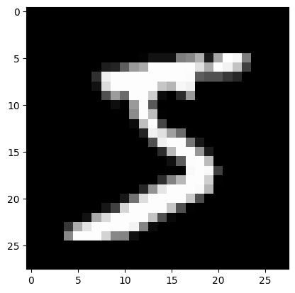
Finally, let’s plot the image we extracted from the dataset and plot it just to get a sense of the kind of data we are dealing with.
import matplotlib.pyplot as plt

print('Sample output:', sample_out)
plt.imshow(tens[0], cmap='gray')

plt.show()
Sample output: 5