Fitting Nonlinear Models#
If you have a dataset and suspects that the data can be modeled effectively with a linear model, then you typically would use linear regression to fit the model. If, however, you think that your data may be best modeled by a nonlinear model, then you would typically use a numerical optimization method like gradient descent.
Creating your own models is a important part of science, and PyTorch allows one to easily mix simple algebraic models with neural network models, allowing them to be trained simultaneously as a single optimization problem. In this section, we will discuss how the problem of fitting a model’s parameters to data can be solved naturally using gradient descent, construct a PyTorch model of the California Housing Dataset’s target variable (median housing price) in terms of its feature variables, construct a PyTorch Dataset object for the California Housing Dataset, and finally use the dataset to train the model.
Several of the constructions we learn in this section (in particular, PyTorch’s Module class, which is used for models, and its Dataset class) add a layer of abstraction and complexity to the goals of this lesson that are not strictly necessary for the kind of optimization we are performing here. However, these classes are used identically in a nonlinear model as they are in a convolutional neural network, and they are far more important in such a case. The simple optimization problem examined in this section provides an introduction to the tools we will need in the next lesson.
How does fitting nonlinear models to data work?#
In the previous section we saw how gradient descent can be used to find the minimum value of a function with respect to its parameters. Specifically, we saw how we could minimize the value of a function \(f(x, y)\) by following the opposite of the function’s gradient. Fitting the parameters of a nonlinear model is essentially the same, but we have to separate the loss function from the model function. To explain this, we should start by formalizing some terms and goals:
Let \(f(x, y; a, b, c)\) be the model function, which predicts fome value \(z = f(x,y; a, b, c)\) in terms of its inputs, \(x\) and \(y\), and its parameters, \(a\), \(b\), and \(c\). As an example, let’s use a model of a 2D symmetric normal distribution: \(f(x, y; \mu_x, \mu_y, \sigma) = \exp\left(\frac{(x - \mu_x)^2 + (y - \mu_y)^2}{2\sigma}\right)\).
Let our dataset contain measured values (with some noise) of both the model’s inputs \(x\) and \(y\) and its associated model output \(z\); let there be \(n\) rows in the dataset, each equivalent to a tuple \((x_i, y_i, z_i)\) (for \(i \in \{0,1,2 ... n-1\})\).
Let \(l_{f}(a,b,c)\) be our loss function, which we are trying to minimize, whose parameters \(a\), \(b\), and \(c\) are identical to those of our model. However, our loss function does not require the model inputs, \(x\) and \(y\) because it will get samples of \(x\) and \(y\) from our dataset.
The overall goal of our optimization is to find the values of \(\mu_x\), \(\mu_y\), and \(\sigma\) that minimize the error between \(f(x, y; \mu_x, \mu_y, \sigma)\) and the \(z\) values observed in our dataset. So, for a row in the dataset \((x_i, y_i, z_i)\), we can define that row’s loss to be \(\left(f(x_i, y_i; \mu_x, \mu_y, \sigma) - z_i\right)^2\).
Note
We use the function \(\left(f(x_i, y_i; \mu_x, \mu_y, \sigma) - z_i\right)^2\) as the loss for a single row \((x_i, y_i, z_i)\) of our dataset. This isn’t the only loss we could have used, however. For example, we could have used \(\left|f(x_i, y_i; \mu_x, \mu_y, \sigma) - z_i\right|\) or \(\log\left|f(x_i, y_i; \mu_x, \mu_y, \sigma) - z_i\right|\); all of these would work because they all have minima when the model’s prediction is equal to the measured \(z\) value. The different loss functions can have non-trivial effects on an oprimization and and are beyond the scope of this lesson. We will typically use what is called the \(L2\) loss function: \((p - m)^2\) where \(p\) is the model prediction and \(m\) is the measured value from the dataset. The L2 loss function is the most common loss function and is in particular appropriate when the noise in the measurement is normal.
Once we’ve defined the loss for a row, we can define the loss for the whole dataset as the sum of the loss for each row. So we can define our loss function as follows:
The above loss function is a little bit more complicated than our previous loss function, but there’s no reason we can’t implement all of this in PyTorch and minimize it just like we did in the previous section.
Example: Psychophysical Functions#
In perceptual psychology, a common paradigm is that a scientist will measure test subject’s response to a stimulus of some kind in terms of some parameter of the stimulus. For example, a scientist who studies hearing, might measure a subject’s ability to detect a sound (their response) in terms of the sound’s volume. In such a case and in many similar perceptual experiments, the probability that a subject detects the sound is in terms of the sound’s intensity can be modeled using what is called a psychometric function. Psychometric functions are typically modeled using sigmoid functions.
This lesson includes a hypothetical dataset in a file called psychophysical_data.csv containing measurements from a hypothetical psychophysics experiment. In this experiment, a human subject sat in front of a computer screen where striped patterns were displayed at various contrasts. These patterns looked like the following images (called gabor patches) with one exception—each was tilted just 4° to either the right or the left.

Over the course of the experiment, the subject was shown 25 different contrasts evenly spaced between 0 and 100%, and they were shown each contrast 40 different times. Each time, they were briefly shown the stimulus image for 200 ms then were asked whether the image had been tilted to the right or the left. If they answer correctly, their response is recorded as True and otherwise is recorded as False.
As researchers studying the perception of contrast, we are interested in making a model of the probability that the subject is able to correctly detect a stimulus given that it has a particular contrast. We will model this as a sigmoid function.
To start with, let’s go ahead and load this data using pandas.
import pandas as pd

psych_data = pd.read_csv('psychophysical_data.csv')
psych_data
| contrast | correct_response | |
|---|---|---|
| 0 | 58.333333 | True |
| 1 | 8.333333 | True |
| 2 | 83.333333 | True |
| 3 | 58.333333 | True |
| 4 | 58.333333 | True |
| ... | ... | ... |
| 995 | 100.000000 | True |
| 996 | 8.333333 | False |
| 997 | 50.000000 | True |
| 998 | 70.833333 | True |
| 999 | 95.833333 | True |
1000 rows × 2 columns
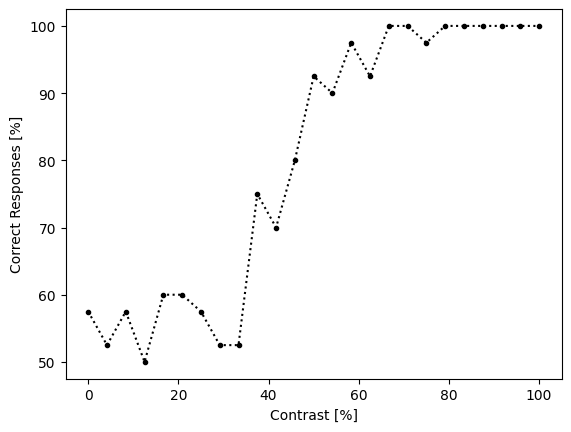
We can see that the dataset is pretty simple; each row records a particular contrast as well as whether the subject responded correctly or not. The contrasts are in a random order, which is how they were presented during the experiment. We might want to theoretically begin by sorting and grouping our dataframe in order to figure out the probability of responding correctly to each contrast.
proportion_correct = psych_data.sort_values(by='contrast').groupby('contrast').mean()
proportion_correct
| correct_response | |
|---|---|
| contrast | |
| 0.000000 | 0.575 |
| 4.166667 | 0.525 |
| 8.333333 | 0.575 |
| 12.500000 | 0.500 |
| 16.666667 | 0.600 |
| 20.833333 | 0.600 |
| 25.000000 | 0.575 |
| 29.166667 | 0.525 |
| 33.333333 | 0.525 |
| 37.500000 | 0.750 |
| 41.666667 | 0.700 |
| 45.833333 | 0.800 |
| 50.000000 | 0.925 |
| 54.166667 | 0.900 |
| 58.333333 | 0.975 |
| 62.500000 | 0.925 |
| 66.666667 | 1.000 |
| 70.833333 | 1.000 |
| 75.000000 | 0.975 |
| 79.166667 | 1.000 |
| 83.333333 | 1.000 |
| 87.500000 | 1.000 |
| 91.666667 | 1.000 |
| 95.833333 | 1.000 |
| 100.000000 | 1.000 |
While we could theoretically extract these probabilities and fit our sigmoid function to it, we will see in a moment that we don’t really need to. However, these data are useful for visualizing the dataset:
import matplotlib.pyplot as plt

x = proportion_correct.index
y = proportion_correct['correct_response']
plt.plot(x, y * 100, 'k.:')
plt.xlabel('Contrast [%]')
plt.ylabel('Correct Responses [%]')

plt.show()
We’re going to fit the dataset using model based on a sigmoid funtion. Sigmoid functions typically have the following form:
Before we define our model, however, we need to split our data into training and test data. We’ll do that with the original set of measurements, not the probability summaries we just produced. We’ll choose a random 30% of rows to be in the test dataset.
# Select a random 80% of rows from the pandas dataframe for the training data:
train_data = psych_data.sample(frac=0.7, random_state=0)
test_data = psych_data.loc[~psych_data.index.isin(train_data.index)]

# Extract contrast (feature) and response (target), and turn them into PyTorch
# tensors:
train_featdata = train_data['contrast'].values
train_targdata = train_data['correct_response'].values

test_featdata = test_data['contrast'].values
test_targdata = test_data['correct_response'].values
Creating a PyTorch Dataset#
PyTorch has its own class for dealing with datasets. While it isn’t strictly necessary for us to use it for this model, it’s good practice for more models that process more complex inputs like convolutional neural networks. Defining a dataset type for the psychophysical data lets it interact with other PyTorch tools that we’ll see later.
To make a PyTorch dataset, we need to overload the Dataset class. This only requires us to write two methods: __len__ and __getitem__; in other words, PyTorch only needs to know how many rows there are in a dataset (__len__) and how to get a single row (__getitem__). The __getitem__ method is expected to return a tuple of (input, output), or possibly (input_1, input_2 ... input_n, output).
import torch
from torch.utils.data import Dataset

# Define a dataset type for our psychophysical ataset.
# We'll expect the training and test subdatasets to be separate dataset
# objects, so we'll design this class to receive as a parameter the rows of
# the dataset and the targets that it includes.
class PsychDataset(Dataset):
    """A PyTorch Dataset implementation of our psychophysical dataset."""
    def __init__(self, features, targets):
        # Convert the features and targets into tensors:
        self.features = torch.tensor(features, dtype=torch.float32)
        self.targets = torch.tensor(targets, dtype=torch.float32)
    def __len__(self):
        return len(self.features)
    def __getitem__(self, idx):
        # Return (model_input, model_output):
        return (self.features[idx], self.targets[idx])

# Make datasets for test and training data:
train_dset = PsychDataset(train_featdata, train_targdata)
test_dset = PsychDataset(test_featdata, test_targdata)
# The datasets should have lengths:
print('train len:', len(train_dset))
print('test len:', len(test_dset))

# Look at one of the entries:
train_dset[10]
train len: 700
test len: 300
(tensor(70.8333), tensor(1.))
Creating the PyTorch model.#
PyTorch also has a class for handling models. It is specifically designed for neural network models, but it is useful for any kind of model, generally. The type is torch.nn.Module.
The Module type only expects its subtypes to define one method: forward, which calculates the model result given a set of inputs. The model parameters should be member variables of the Module subtype (collections of parameters like lists of tensors are also fine), and the Module will handle various aspects of manipulating these parameters like saving them to or loading them from a file.
The Module class does have some idiosyncrasies. First, it expects that you always call the superclass’s __init__ method as the first step in your subclass’s __init__ method. Second, it expects all input tensors (i.e., inputs to the forward method) to conform to a particular shape: they must start with dimensions representing batch and channel.
To explain what the batch and channel are, it’s easiest to think of the the inputs for a convolutional neural network (CNN) that is trained using traditional RGB images as inputs. Each image has 3 channels (red, green, and blue), some number of rows (\(N\)), and some number of columns (\(M\)). An RGB image would usually be stored in an array or tensor whose shape is (N, M, 3)—i.e., rows, columns, channels. PyTorch wants the first two dimensions to correspond to batch and channel, though, so the shape of an image input to such a CNN is expected to be (B, 3, N, M) where B is the “batch” size. The batch size is the number of samples being computed by the model at once, and so can be any number, including 1. The reason there is a batch size is because for many large models or models that are trained on large inputs, the entire dataset cannot fit in memory at once, and so the loss function cannot be calculated over the whole dataset during one step of the optimizer. Instead it uses a random subset of the dataset during each step. We will see more examples of batch sizes in the next lesson.
In the case of our training, the batch size is just the number of rows the model is calculating and the number of channels is just the number of features; each feature is a single number, so instead of (B, C, N, M), we have just (B, C). We will use the entire dataset as a single batch.
The batch size used during training is a hyperparameter of the model training; in theory it should not have a large effect on the optimal point that is found by the optimization algorithm, but it can substantially affect the speed at which the training finds that point.
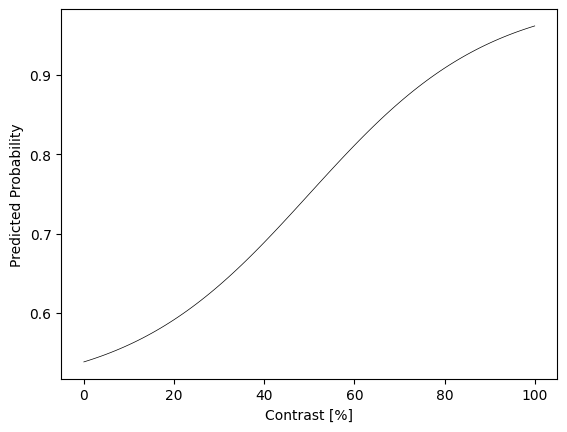
Let’s create an implementation of our model; PyTorch includes a builtin sigmoid function, so most of the code in this model is boilerplate PyTorch code.
from torch.nn import Module, Parameter

def psi(x):
    return 0.5 * (1 + torch.sigmoid(x))

class PsychometricModel(Module):
    """A model of the probability of correctly detecting the direction of tilt
    of a gabor patch in terms of the patch's contrast.

    The model has two parameter tensors, each with 1 element: a and c0.
    The model expects inputs with 1 channel, each of which is a single real
    number.
    The form of the model is:
        sigmoid(a * (contrast - c0))
    """
    def __init__(self, a=0.05, c0=50.0):
        # Start with the superclass init:
        super().__init__()
        # We declare the parameters using the Parameter type.
        # We ccould hoose the initial state as a random number, but for
        # these, we'll use constant guesses (0).
        # Parameters always get requires_grad set to True when they are
        # created, so we don't need to specify it.
        self.a = Parameter(torch.tensor(a))
        self.c0 = Parameter(torch.tensor(c0))
    def forward(self, contrasts):
        # There is just one number per batch in the features, so we can just
        # flatten it into a vector of contrasts.
        contrasts = torch.flatten(contrasts)
        # Calculate the model:
        (a,c0) = (self.a, self.c0)
        return psi(a * (contrasts - c0))

# Declare a model:
model = PsychometricModel()

# Plot a sample:
contrast_range = torch.arange(101)
pred_prob = model(contrast_range[None,:]).detach().numpy()
plt.plot(contrast_range, pred_prob.flat, 'k-', lw=0.5)
plt.xlabel('Contrast [%]')
plt.ylabel('Predicted Probability')

plt.show()
Now that we’ve created a model and a dataset, we can use the dataset to train the model. To do this we use an intermediate class called a DataLoader. The DataLoader class is in charge of choosing elements from the dataset and feeding them to the model during training. The DataLoader is the class that handles the batch sizes, which in our case will just be the size of the dataset. When we iterate over a DataLoader, it returns tuples containing batches of inputs and outputs ready to be passed to the model.
from torch.utils.data import DataLoader

train_dloader = DataLoader(train_dset, batch_size=len(train_dset))
test_dloader = DataLoader(test_dset, batch_size=len(test_dset))
Before we can start minimizing, we also need to declare our loss function. A common loss function is one called the mean squared error (MSE) loss, but in our case, we are actually dealing with classes and probabilities. The data contains classes (correct or incorrect) that we have translated into the values 1 (correct) and 0 (incorrect). The model predicts a probability of each class, given a particular contrast. For such a situation, a better loss function is the binary cross entropy (BCE) loss, which is specifically useful for this kind of classification problem. The BCE loss increases if the predicted probability of a 1 decreases or if the predicted probability of a 0 increases. It is defined as:
keeping in mind that the value of the target (\(t\)) will always be a 1 or a 0 and the value of \(p\) is a probability. PyTorch includes a built-in BCE loss utility that we will use.
from torch.nn import BCELoss

loss = BCELoss()
We can now set up our training loop. This loop will be almost the same as the minimization loop in the previous section, but instead of just calling a function f(x,y) it will call the model to produce a prediction then calculate a loss using our loss function. The loss is what we will minimize.
# Hyperparameters:
n_steps = 20
lr = 0.01


# Now that we've declared our hyperparameters, let's declare our model.
# This will generate new random starting parameters when run.
model = PsychometricModel()

# Next, we can declare an optimizer.
# We'll continue to use the optimizer SGD. SGD needs to know our model
# parameters, but the `model.parameters()` method will return them for us.
optimizer = torch.optim.SGD(model.parameters(), lr=lr)

# Declare our loss function:
loss_fn = torch.nn.BCELoss()

# Now we can take several optimization steps:
for step_number in range(n_steps):
    # In each model we basically do two things: (1) train the model with the
    # training data then (2) test the model with the testing data.
    # When training we want to put the model into training mode.
    model.train()
    # During each step, we will iterate over the training dataloader;
    # because our batch size is the same size as the dataset there will only
    # be one entry to iterate over, but that's fine.
    for (inputs, targets) in train_dloader:
        # We're starting a new step, so we reset the gradients.
        optimizer.zero_grad()
        # Calculate the model prediction for these inputs.
        preds = model(inputs)
        # Calculate the loss between the prediction and the actual outputs.
        train_loss = loss_fn(preds, targets)
        # Have PyTorch backward-propagate the gradients.
        train_loss.backward()
        # Have the optimizer take a step:
        optimizer.step()
        # Print the batch's R2 value:
        var = torch.var(targets)
        mse = torch.mean((preds - targets)**2)
        train_r2 = 1 - mse/var
    # Now that we've finished training, put the model back in evaluation mode.
    model.eval()
    # Evaluate the model using the test data.
    for (inputs, targets) in test_dloader:
        preds = model(inputs)
        test_loss = loss_fn(preds, targets)
        var = torch.var(targets)
        mse = torch.mean((preds - targets)**2)
        test_r2 = 1 - mse/var
    # Print something about this step:
    print(f"Step {step_number:3d}  train r2={train_r2:6.3f} loss={train_loss.detach():6.3f} ;  test r2={test_r2:6.3f} loss={test_loss.detach():6.3f}")
# After the optimizer has run, print out what it's found:
print("Final result:")
print(f"  train loss = ", float(train_loss.detach()))
print(f"   test loss = ", float(test_loss.detach()))
Step   0  train r2= 0.181 loss= 0.390 ;  test r2= 0.218 loss= 0.432
Step   1  train r2= 0.189 loss= 0.382 ;  test r2= 0.224 loss= 0.427
Step   2  train r2= 0.192 loss= 0.378 ;  test r2= 0.227 loss= 0.424
Step   3  train r2= 0.194 loss= 0.375 ;  test r2= 0.229 loss= 0.421
Step   4  train r2= 0.196 loss= 0.373 ;  test r2= 0.231 loss= 0.419
Step   5  train r2= 0.196 loss= 0.372 ;  test r2= 0.232 loss= 0.418
Step   6  train r2= 0.197 loss= 0.370 ;  test r2= 0.232 loss= 0.417
Step   7  train r2= 0.197 loss= 0.369 ;  test r2= 0.233 loss= 0.416
Step   8  train r2= 0.197 loss= 0.368 ;  test r2= 0.234 loss= 0.415
Step   9  train r2= 0.197 loss= 0.368 ;  test r2= 0.234 loss= 0.414
Step  10  train r2= 0.198 loss= 0.367 ;  test r2= 0.234 loss= 0.414
Step  11  train r2= 0.198 loss= 0.367 ;  test r2= 0.235 loss= 0.413
Step  12  train r2= 0.198 loss= 0.366 ;  test r2= 0.235 loss= 0.413
Step  13  train r2= 0.198 loss= 0.366 ;  test r2= 0.235 loss= 0.412
Step  14  train r2= 0.198 loss= 0.365 ;  test r2= 0.235 loss= 0.412
Step  15  train r2= 0.198 loss= 0.365 ;  test r2= 0.235 loss= 0.412
Step  16  train r2= 0.197 loss= 0.365 ;  test r2= 0.235 loss= 0.412
Step  17  train r2= 0.197 loss= 0.364 ;  test r2= 0.235 loss= 0.411
Step  18  train r2= 0.197 loss= 0.364 ;  test r2= 0.236 loss= 0.411
Step  19  train r2= 0.197 loss= 0.364 ;  test r2= 0.236 loss= 0.411
Final result:
  train loss =  0.3639899790287018
   test loss =  0.4108993411064148
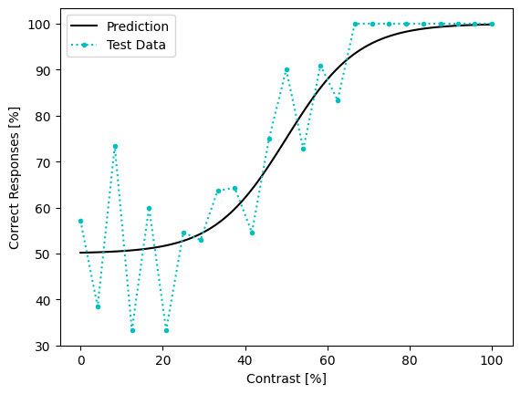
To see how well our fitting did, let’s take a look at the results and compare it to the test dataset.
# Plot model prediction:
pred_prob = model(contrast_range[None,:]).detach().numpy()
plt.plot(contrast_range, (pred_prob * 100).flat, 'k-', label='Prediction')

# Plot prop correct from dataset:
propcorr = test_data.sort_values(by='contrast').groupby('contrast').mean()
x = propcorr.index
y = propcorr['correct_response']
plt.plot(x, y * 100, 'c.:', label='Test Data')
plt.xlabel('Contrast [%]')
plt.ylabel('Correct Responses [%]')
plt.legend()

plt.show()