Optimization and Gradient Descent

Optimization is a broad topic in machine learning; we will focus on a specific (but large and powerful) subset of optimization in which an algorithm attempts to learn the parameters of a function that minimize its (continuous real-valued) output. If one can perform this kind of optimization, one can also use it to learn the parameters of a model that best explains a set of data. PyTorch excels at both of these methods, which are the foundation of the next lesson on neural networks. We’ll start by examining the former then use it to construct the latter method in the next section.

How does gradient descent optimization work?

The basic idea of gradient descent is that the gradient of a function points in the direction it is increasing the fastest and its opposite is the direction in which it decreases the fastest, so if you make a guess at the parameters that minimize the function then calculate the gradient at that point, it tells you the direction of a point that’s closer to the minimum. You can then take a small step in that direction and repeat the process until you’re as close as you need to be.

We’ll unpack the description of gradient descent immediately above using a simple example. Suppose we are looking for the minimum of the following function:

\[ f(x, y) = (x - 1)^2 + 4(y + 1)^2 + \frac{x y}{2} \]

This function doesn’t mean anything to us in particular, but we’ll use it as an example. In this example, \(f\) is our loss function—i.e., the real-valued continuous function that we are trying to minimize. Here, \(x\) and \(y\) are the parameters that we are learning.

Example: finding the minimum of a simple function.

We’ll start by implementing the function \(f\) (from above) in Python code.

import torch

# This function will work fine with PyTorch tensors or with NumPy arrays
# as long as both x and y are the same type.
def f(x, y):
    return (x - 1)**2 + 4*(y + 1)**2 + x*y/2

# Test that it works:
f(3, 3)

72.5

Notice that we can make tensors out of individual numbers (individual numbers are just rank-0 tensors), and when we perform calculations using these tensor numbers, they yield tensor numbers as well.

x = torch.tensor(3.0)
y = torch.tensor(3.0)

f(x, y)

tensor(72.5000)

The requires_grad option enables gradient calculation.

Recall that the torch.tensor function and similar tensor-creation functions like torch.ones and torch.zeros accept an optional argument requires_grad. This option tells a tensor that it’s a parameter to a function involved in some kind of optimization, and so the gradient of this value with respect to some computed value may be required. Let’s look at an example of this.

x = torch.tensor(3.0, requires_grad=True)
y = torch.tensor(3.0, requires_grad=True)

# Calculate the value of the function:
z = f(x, y)

# Ask PyTorch to backward-propagate the gradient of z to its parameters
# (this calculates the gradient of z with respect to its parameters x and y
# then tells those parameters what their components of the gradients are).
z.backward()

# Now we can examine the gradient of f(x,y) with respect to x and y:
print('∂f/∂x =', x.grad)
print('∂f/∂y =', y.grad)

∂f/∂x = tensor(5.5000)
∂f/∂y = tensor(33.5000)

The requires_grad option can be very powerful and is required for all parameters in PyTorch optimizations. It does induce a few changes to the way that that one interacts with the tensor, however. These changes are required because PyTorch needs to carefully keep track of all the calculations that result from any tensors that require gradients—if a tensor involved in these calculations gets updated outside of PyTorch’s ecosystem, it can lose track of critical parts of the calculation and create incorrect gradients.

Primarily, when requires_grad is enabled, accessing the NumPy array of a PyTorch tensor requires an extra step, and in-place operations become illegal.

# For normal tensors of single numbers, we can update the tensor by using an
# empty tuple in the setitem paradigm (tensor[()] = new_value):
tens = torch.tensor(0.0)
tens[()] = 1.0
print('tens:', tens)

# But for a tensor that requires gradient, one cannot update the tensor
# directly because this would ruin the gradient tracking.
x[()] = 10  # This will raise an error.

tens: tensor(1.)

---------------------------------------------------------------------------
RuntimeError                              Traceback (most recent call last)
Cell In[4], line 9
      5 print('tens:', tens)
      7 # But for a tensor that requires gradient, one cannot update the tensor
      8 # directly because this would ruin the gradient tracking.
----> 9 x[()] = 10  # This will raise an error.

RuntimeError: a leaf Variable that requires grad is being used in an in-place operation.

# For a normal tensor, we can access it's NumPy array using the x.numpy()
# method.
tens_np = tens.numpy()
print('tens_np:', tens_np)

# For a tensor that requires gradient, this will raise an error, because
# editing the NumPy tensor would ruin the gradient tracking (and once PyTorch
# returns the array, it can't stop you from editing it).
print(x.numpy())  # This will raise an error.

tens_np: 1.0

---------------------------------------------------------------------------
RuntimeError                              Traceback (most recent call last)
Cell In[5], line 9
      4 print('tens_np:', tens_np)
      6 # For a tensor that requires gradient, this will raise an error, because
      7 # editing the NumPy tensor would ruin the gradient tracking (and once PyTorch
      8 # returns the array, it can't stop you from editing it).
----> 9 print(x.numpy())  # This will raise an error.

RuntimeError: Can't call numpy() on Tensor that requires grad. Use tensor.detach().numpy() instead.

# The same is true of any tensor involved in gradient tracking; because z is
# the result of a computation that included a tensor with requires_grad=True,
# z cannot be directly accessed or edited either.
print(z.numpy())  # This will raise an error.

---------------------------------------------------------------------------
RuntimeError                              Traceback (most recent call last)
Cell In[6], line 4
      1 # The same is true of any tensor involved in gradient tracking; because z is
      2 # the result of a computation that included a tensor with requires_grad=True,
      3 # z cannot be directly accessed or edited either.
----> 4 print(z.numpy())  # This will raise an error.

RuntimeError: Can't call numpy() on Tensor that requires grad. Use tensor.detach().numpy() instead.

# As the error message suggests, we have to detach a tensor that is part of
# any gradient tracking before we extract a numpy array.
print(x.detach().numpy())

3.0

The detach() method can be used to make a duplicate PyTorch tensor that no longer has requires_grad set to True.

Warning

Although x.detach() returns a new PyTorch tensor that has been detached from the gradient tracking system, it still uses the same memory under the hood to store the tensor elements as the original PyTorch tensor. This means that if you edit the detached tensor or its associated NumPy array, it can produce errors when gradients are computed. If you plan to edit these arrays you should copy them first!

The Optimization Loop

To perform the minimization, we’ll start by making a guess as to \(x\) and \(y\) values that yield the minimum. (It may not be a very good guess.) We’ll create an optimizer (a PyTorch class) that manages the state of the optimization. We’ll then take repeated steps toward the minimum using the gradient. (PyTorch mostly does this automatically for us.) In each step, we’ll perform a few sub-steps:

1. Calculate the value of the function at \(x\) and \(y\) (z = f(x, y)). The value z that is returned is a PyTorch tensor.

2. Calculate and propogate the gradient backward from z to its parameters x and y. PyTorch does this step for us via the method z.backward().

3. Tell the optimizer to take a step. PyTorch does the work in this step, which involves updating all of the parameters (x and y in this case), to be a little closer to the minimum.

Note

The number of steps to take is a hyperparemter of the optimization. A larger number of steps will usually result in a better optimization, but the improvement in the optimization usually diminishes with each step.

Alternatively, one can use a heuristic to decide when to stop, such as choosing to take steps until the change in the function value is smaller than some fixed value.

# There are a few hyperparameters we can declare ahead of time.

# The number of steps determins how many minimization steps we take.
n_steps = 50

# The learning rate is essentially a knob we can turn to try to speed up or
# slow down the optimization. A higher learning rate means that the optimizer
# takes larger steps along the gradient; a lower learning rate means that it
# takes smaller steps. Small steps converge more slowly, but if you take too
# large of a step you can pass the minimum and potentially get farther away.
# The best learning rate will depend on the optimizer and the function being
# optimized, so it often has to be found experimentally.
lr = 0.1

# Now that we've declared our hyperparameters, let's declare our parameters.
x = torch.tensor(3.0, requires_grad=True)
y = torch.tensor(3.0, requires_grad=True)

# Next, we can declare an optimizer.
# We'll use the optimizer SGD: stochastic gradient descent.
# The "stochastic" refers to the way it handles training when a dataset is
# involved and does not indicate that this method is stochastic in this case.
# The optimizer will manage the steps and updating the parameters during them.
# Because of this we have to tell it the parameters and the learning rate.
optimizer = torch.optim.SGD([x, y], lr=lr)

# Now we can take several optimization steps:
for step_number in range(n_steps):
    # We're starting a new step, so we reset the gradients.
    optimizer.zero_grad()
    # Calculate the function value at these parameters.
    z = f(x, y)
    # Have PyTorch backward-propagate the gradients.
    z.backward()
    # If the norm of the gradient is less than 1e-5, we finish early.
    if torch.hypot(x.grad, y.grad) < 1e-4:
        break
    # Print a message about this step:
    print("Step number", step_number)
    print("  x = ", float(x), ";  ∂f/∂x = ", float(x.grad))
    print("  y = ", float(y), ";  ∂f/∂y = ", float(y.grad))
    print("  z = ", float(z))
    # Have the optimizer take a step:
    optimizer.step()

# After the optimizer has run, print out what it's found:
print("Final result:")
print(f"  f({float(x)}, {float(y)}) = {float(z)}")

Step number 0
  x =  3.0 ;  ∂f/∂x =  5.5
  y =  3.0 ;  ∂f/∂y =  33.5
  z =  72.5
Step number 1
  x =  2.450000047683716 ;  ∂f/∂x =  2.7250001430511475
  y =  -0.3500000536441803 ;  ∂f/∂y =  6.424999713897705
  z =  3.3637499809265137
Step number 2
  x =  2.177500009536743 ;  ∂f/∂x =  1.8587499856948853
  y =  -0.9925000071525574 ;  ∂f/∂y =  1.1487499475479126
  z =  0.30614686012268066
Step number 3
  x =  1.9916249513626099 ;  ∂f/∂x =  1.4295623302459717
  y =  -1.1073750257492065 ;  ∂f/∂y =  0.1368122696876526
  z =  -0.07330024242401123
Step number 4
  x =  1.8486686944961548 ;  ∂f/∂x =  1.1368093490600586
  y =  -1.1210561990737915 ;  ∂f/∂y =  -0.04411524534225464
  z =  -0.2573738098144531
Step number 5
  x =  1.734987735748291 ;  ∂f/∂x =  0.9116531610488892
  y =  -1.1166446208953857 ;  ∂f/∂y =  -0.06566309928894043
  z =  -0.3740515112876892
Step number 6
  x =  1.643822431564331 ;  ∂f/∂x =  0.7326056957244873
  y =  -1.1100783348083496 ;  ∂f/∂y =  -0.05871546268463135
  z =  -0.449409544467926
Step number 7
  x =  1.5705618858337402 ;  ∂f/∂x =  0.5890203714370728
  y =  -1.1042068004608154 ;  ∂f/∂y =  -0.04837346076965332
  z =  -0.4981354773044586
Step number 8
  x =  1.511659860610962 ;  ∂f/∂x =  0.4736350178718567
  y =  -1.0993694067001343 ;  ∂f/∂y =  -0.03912532329559326
  z =  -0.5296434164047241
Step number 9
  x =  1.4642963409423828 ;  ∂f/∂x =  0.3808642625808716
  y =  -1.095456838607788 ;  ∂f/∂y =  -0.03150653839111328
  z =  -0.5500175952911377
Step number 10
  x =  1.4262099266052246 ;  ∂f/∂x =  0.30626678466796875
  y =  -1.092306137084961 ;  ∂f/∂y =  -0.025344133377075195
  z =  -0.5631923675537109
Step number 11
  x =  1.3955832719802856 ;  ∂f/∂x =  0.24628067016601562
  y =  -1.0897717475891113 ;  ∂f/∂y =  -0.020382344722747803
  z =  -0.5717116594314575
Step number 12
  x =  1.370955228805542 ;  ∂f/∂x =  0.19804370403289795
  y =  -1.087733507156372 ;  ∂f/∂y =  -0.016390442848205566
  z =  -0.5772204995155334
Step number 13
  x =  1.3511508703231812 ;  ∂f/∂x =  0.15925449132919312
  y =  -1.0860944986343384 ;  ∂f/∂y =  -0.013180553913116455
  z =  -0.5807827711105347
Step number 14
  x =  1.3352254629135132 ;  ∂f/∂x =  0.12806272506713867
  y =  -1.0847764015197754 ;  ∂f/∂y =  -0.010598480701446533
  z =  -0.5830863118171692
Step number 15
  x =  1.3224191665649414 ;  ∂f/∂x =  0.10298007726669312
  y =  -1.0837165117263794 ;  ∂f/∂y =  -0.008522510528564453
  z =  -0.5845758318901062
Step number 16
  x =  1.3121211528778076 ;  ∂f/∂x =  0.0828101634979248
  y =  -1.0828642845153809 ;  ∂f/∂y =  -0.006853699684143066
  z =  -0.5855389833450317
Step number 17
  x =  1.303840160369873 ;  ∂f/∂x =  0.06659084558486938
  y =  -1.0821789503097534 ;  ∂f/∂y =  -0.00551152229309082
  z =  -0.5861617922782898
Step number 18
  x =  1.2971811294555664 ;  ∂f/∂x =  0.053548336029052734
  y =  -1.0816278457641602 ;  ∂f/∂y =  -0.004432201385498047
  z =  -0.5865645408630371
Step number 19
  x =  1.2918262481689453 ;  ∂f/∂x =  0.04306018352508545
  y =  -1.0811846256256104 ;  ∂f/∂y =  -0.0035638809204101562
  z =  -0.5868250131607056
Step number 20
  x =  1.287520170211792 ;  ∂f/∂x =  0.03462624549865723
  y =  -1.0808281898498535 ;  ∂f/∂y =  -0.002865433692932129
  z =  -0.586993396282196
Step number 21
  x =  1.2840574979782104 ;  ∂f/∂x =  0.02784419059753418
  y =  -1.0805416107177734 ;  ∂f/∂y =  -0.0023041367530822754
  z =  -0.5871022939682007
Step number 22
  x =  1.2812731266021729 ;  ∂f/∂x =  0.022390663623809814
  y =  -1.0803111791610718 ;  ∂f/∂y =  -0.001852869987487793
  z =  -0.5871726870536804
Step number 23
  x =  1.2790340185165405 ;  ∂f/∂x =  0.018005073070526123
  y =  -1.0801259279251099 ;  ∂f/∂y =  -0.0014904141426086426
  z =  -0.5872182250022888
Step number 24
  x =  1.2772334814071655 ;  ∂f/∂x =  0.014478504657745361
  y =  -1.0799769163131714 ;  ∂f/∂y =  -0.00119858980178833
  z =  -0.5872477293014526
Step number 25
  x =  1.2757856845855713 ;  ∂f/∂x =  0.011642813682556152
  y =  -1.0798571109771729 ;  ∂f/∂y =  -0.000964045524597168
  z =  -0.587266743183136
Step number 26
  x =  1.2746213674545288 ;  ∂f/∂x =  0.009362399578094482
  y =  -1.0797606706619263 ;  ∂f/∂y =  -0.000774681568145752
  z =  -0.5872790813446045
Step number 27
  x =  1.273685097694397 ;  ∂f/∂x =  0.0075286030769348145
  y =  -1.0796831846237183 ;  ∂f/∂y =  -0.0006229281425476074
  z =  -0.5872870683670044
Step number 28
  x =  1.2729322910308838 ;  ∂f/∂x =  0.0060541629791259766
  y =  -1.0796208381652832 ;  ∂f/∂y =  -0.0005005598068237305
  z =  -0.5872921943664551
Step number 29
  x =  1.2723268270492554 ;  ∂f/∂x =  0.004868268966674805
  y =  -1.0795707702636719 ;  ∂f/∂y =  -0.00040274858474731445
  z =  -0.5872955322265625
Step number 30
  x =  1.27183997631073 ;  ∂f/∂x =  0.0039147138595581055
  y =  -1.0795304775238037 ;  ∂f/∂y =  -0.00032383203506469727
  z =  -0.5872976779937744
Step number 31
  x =  1.2714484930038452 ;  ∂f/∂x =  0.0031479597091674805
  y =  -1.079498052597046 ;  ∂f/∂y =  -0.0002601742744445801
  z =  -0.5872990489006042
Step number 32
  x =  1.2711336612701416 ;  ∂f/∂x =  0.002531290054321289
  y =  -1.0794720649719238 ;  ∂f/∂y =  -0.00020968914031982422
  z =  -0.5872999429702759
Step number 33
  x =  1.2708805799484253 ;  ∂f/∂x =  0.0020356178283691406
  y =  -1.079451084136963 ;  ∂f/∂y =  -0.00016838312149047852
  z =  -0.5873005390167236
Step number 34
  x =  1.2706769704818726 ;  ∂f/∂x =  0.001636803150177002
  y =  -1.0794342756271362 ;  ∂f/∂y =  -0.00013571977615356445
  z =  -0.5873008966445923
Step number 35
  x =  1.2705132961273193 ;  ∂f/∂x =  0.0013162493705749512
  y =  -1.0794206857681274 ;  ∂f/∂y =  -0.00010883808135986328
  z =  -0.5873011350631714
Step number 36
  x =  1.2703816890716553 ;  ∂f/∂x =  0.0010584592819213867
  y =  -1.0794098377227783 ;  ∂f/∂y =  -8.785724639892578e-05
  z =  -0.5873013138771057
Step number 37
  x =  1.2702758312225342 ;  ∂f/∂x =  0.0008511543273925781
  y =  -1.0794010162353516 ;  ∂f/∂y =  -7.021427154541016e-05
  z =  -0.5873013734817505
Step number 38
  x =  1.270190715789795 ;  ∂f/∂x =  0.0006844401359558105
  y =  -1.079393982887268 ;  ∂f/∂y =  -5.650520324707031e-05
  z =  -0.5873014330863953
Step number 39
  x =  1.2701222896575928 ;  ∂f/∂x =  0.000550389289855957
  y =  -1.0793883800506592 ;  ∂f/∂y =  -4.589557647705078e-05
  z =  -0.58730149269104
Step number 40
  x =  1.2700672149658203 ;  ∂f/∂x =  0.0004425644874572754
  y =  -1.0793837308883667 ;  ∂f/∂y =  -3.62396240234375e-05
  z =  -0.5873015522956848
Step number 41
  x =  1.270022988319397 ;  ∂f/∂x =  0.0003558993339538574
  y =  -1.0793801546096802 ;  ∂f/∂y =  -2.9742717742919922e-05
  z =  -0.5873015522956848
Step number 42
  x =  1.2699873447418213 ;  ∂f/∂x =  0.000286102294921875
  y =  -1.0793771743774414 ;  ∂f/∂y =  -2.372264862060547e-05
  z =  -0.5873015522956848
Step number 43
  x =  1.269958734512329 ;  ∂f/∂x =  0.0002300739288330078
  y =  -1.0793747901916504 ;  ∂f/∂y =  -1.895427703857422e-05
  z =  -0.5873015522956848
Step number 44
  x =  1.2699357271194458 ;  ∂f/∂x =  0.0001850128173828125
  y =  -1.0793728828430176 ;  ∂f/∂y =  -1.519918441772461e-05
  z =  -0.5873016119003296
Step number 45
  x =  1.2699172496795654 ;  ∂f/∂x =  0.0001488327980041504
  y =  -1.0793713331222534 ;  ∂f/∂y =  -1.2040138244628906e-05
  z =  -0.5873016119003296
Step number 46
  x =  1.2699023485183716 ;  ∂f/∂x =  0.00011962652206420898
  y =  -1.079370141029358 ;  ∂f/∂y =  -9.953975677490234e-06
  z =  -0.5873015522956848
Final result:
  f(1.2698904275894165, -1.0793691873550415) = -0.5873015522956848

/tmp/ipykernel_2474/1998003620.py:40: UserWarning: Converting a tensor with requires_grad=True to a scalar may lead to unexpected behavior.
Consider using tensor.detach() first. (Triggered internally at /pytorch/torch/csrc/autograd/generated/python_variable_methods.cpp:836.)
  print("  x = ", float(x), ";  ∂f/∂x = ", float(x.grad))

Effects of the learning rate parameter.

We can try running the above code-block with different hyperparameters to get a sense of their impact. Try running the above block using a high learning rate (lr=0.5) and a low learning rate (lr=0.01).

With lr=0.01, the optimization works fine, but it doesn’t finish. It gets closer to the minimum, but it doesn’t reach the minimum value found with lr=0.1.

With lr=0.5 the optimization actually diverges! This means that it takes steps so large that they go so past the minimum to a point that’s higher than the start point.

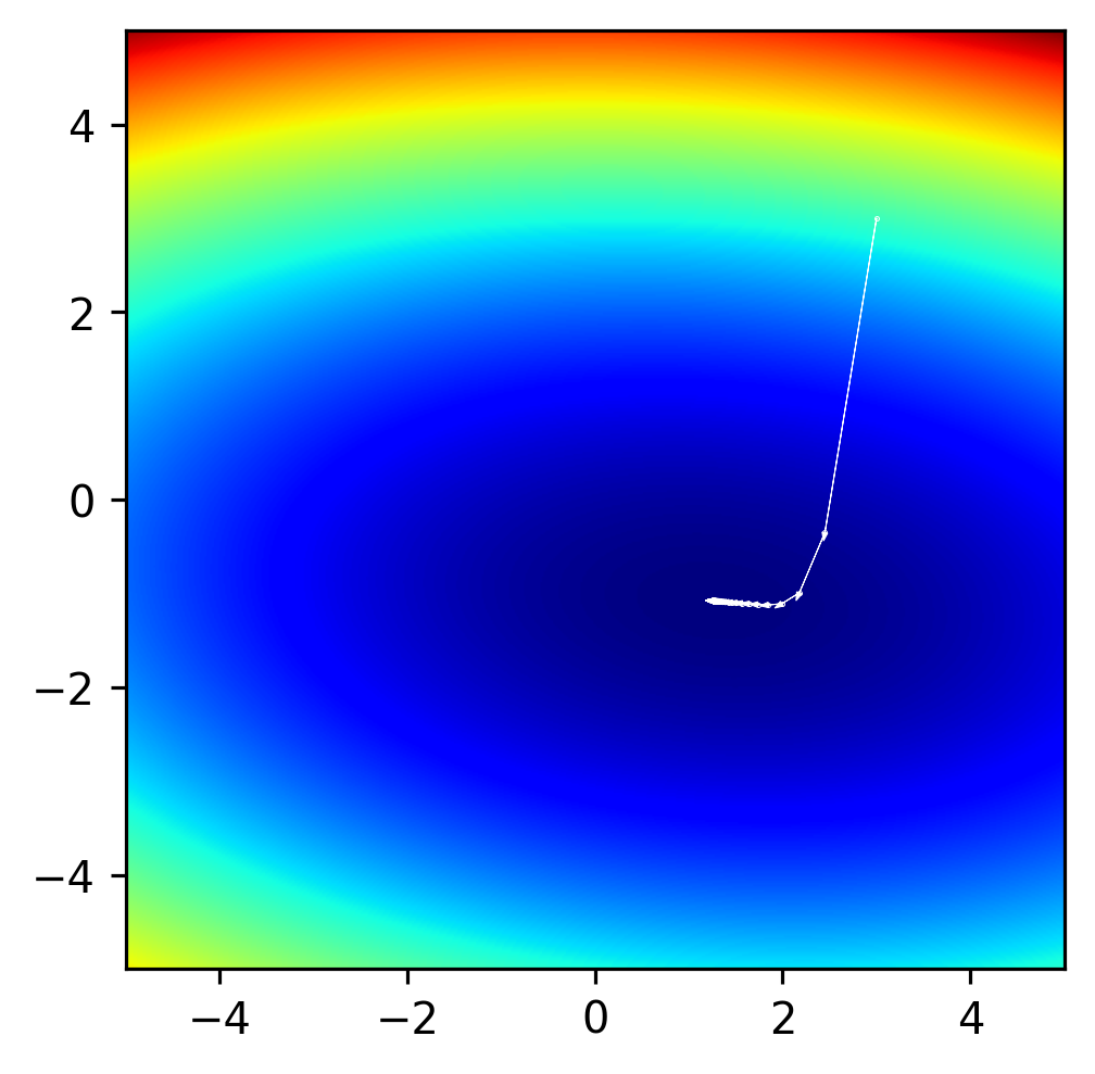
To get a better sense for what these mean, let’s make some plots of the steps that the optimizer takes. Try running this with different lr parameters.

import matplotlib.pyplot as plt
import numpy as np

# Declare our hyperparameters:
n_steps = 50
lr = 0.1

# Now the parameters:
x = torch.tensor(3.0, requires_grad=True)
y = torch.tensor(3.0, requires_grad=True)

# Now the optimizer:
optimizer = torch.optim.SGD([x, y], lr=lr)

# Now we set up a pyplot figure.
(fig,ax) = plt.subplots(1, 1, figsize=(3,3), dpi=288)
fig.subplots_adjust(0, 0, 1, 1, 0, 0)
# Make an image of the function itself and plot it as the background.
(x_im, y_im) = np.meshgrid(
    np.linspace(-5,5,512),
    np.linspace(-5,5,512),
    indexing='xy')
z_im = f(x_im, y_im)
ax.imshow(z_im, cmap='jet', zorder=-1, extent=(-5,5,5,-5))
ax.invert_yaxis()

# Now we can take several optimization steps:
for step_number in range(n_steps):
    # We're starting a new step, so we reset the gradients.
    optimizer.zero_grad()
    # Calculate the function value at these parameters.
    z = f(x, y)
    # Have PyTorch backward-propagate the gradients.
    z.backward()
    # Plot the points and the gradients:
    (x_np, y_np) = (x.detach().numpy(), y.detach().numpy())
    (x_np, y_np) = (np.array(x_np), np.array(y_np))
    ax.plot(x_np, y_np, 'w.', ms=0.5)
    # If the norm of the gradient is less than 1e-5, we finish early.
    if torch.hypot(x.grad, y.grad) < 1e-4:
        break
    # Have the optimizer take a step:
    optimizer.step()
    # Plot the arrow from the previous to this point.
    dx_np = x.detach().numpy() - x_np
    dy_np = y.detach().numpy() - y_np
    ax.arrow(x_np, y_np, dx_np, dy_np, color='w', lw=0.25, head_width=0.06)

# After the optimizer has run, show the steps:
ax.set_xlim([-5,5])
ax.set_ylim([-5,5])
plt.show()

Another Example: The problem of local minima.

Let’s examine a different function. We’ll use essentially the same optimization loop but will define a slightly different function:

\[ g(x, y) = \left((x + 1)^2 + (y + 1)^2\right) \left((x - 3)^2 + (y - 3)^2 + 1\right) \]

Let’s defint this function then run our optimization again.

def g(x, y):
    return ((x + 1)**2 + (y + 1)**2) * ((x - 3)**2 + (y - 3)**2 + 1)

# Declare our hyperparameters:
n_steps = 50
lr = 0.005  # This function is different and needs a lower learning rate.

# Now the parameters; we'll start at slightly different position this time.
x = torch.tensor(3.5, requires_grad=True)
y = torch.tensor(4.0, requires_grad=True)

# Now the optimizer:
optimizer = torch.optim.SGD([x, y], lr=lr)

# Now we set up a pyplot figure.
(fig,ax) = plt.subplots(1, 1, figsize=(3,3), dpi=288)
fig.subplots_adjust(0, 0, 1, 1, 0, 0)
# Make an image of the function itself and plot it as the background.
(x_im, y_im) = np.meshgrid(
    np.linspace(-5,5,512),
    np.linspace(-5,5,512),
    indexing='xy')
z_im = g(x_im, y_im)
# We can add a vmax to make sure our visualization captures the part of the
# image that is of interest to us.
ax.imshow(z_im, cmap='jet', zorder=-1, extent=(-5,5,5,-5), vmax=500)
ax.invert_yaxis()

# Now we can take several optimization steps:
for step_number in range(n_steps):
    # We're starting a new step, so we reset the gradients.
    optimizer.zero_grad()
    # Calculate the function value at these parameters.
    z = g(x, y)
    # Have PyTorch backward-propagate the gradients.
    z.backward()
    # Plot the points and the gradients:
    (x_np, y_np) = (x.detach().numpy(), y.detach().numpy())
    (x_np, y_np) = (np.array(x_np), np.array(y_np))
    ax.plot(x_np, y_np, 'w.', ms=0.5)
    # If the norm of the gradient is less than 1e-5, we finish early.
    if torch.hypot(x.grad, y.grad) < 1e-4:
        break
    # Have the optimizer take a step:
    optimizer.step()
    # Plot the arrow from the previous to this point.
    dx_np = x.detach().numpy() - x_np
    dy_np = y.detach().numpy() - y_np
    ax.arrow(x_np, y_np, dx_np, dy_np, color='w', lw=0.25, head_width=0.06)

# After the optimizer has run, show the steps:
ax.set_xlim([-5,5])
ax.set_ylim([-5,5])
plt.show()

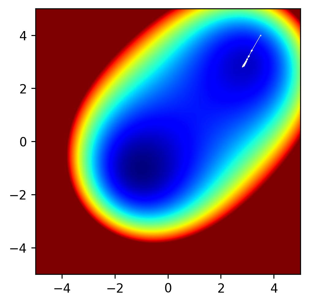
Clearly in the above example, the method found a minimum value, but there’s another minimum value in this function, and it’s lower than the minimum that the optimization method found. What if we change the initial parameters x and y to have a start value closer to the other minimum?

Local minima are an issue in many optimization problems. In some cases, it can be proven that a global minimum has been found, but in many cases it cannot be. One strategy for avoiding local minima is to fit a function many times and to use, as the final result, whatever lowest value was achieved across all runs. Of course, this is quite time consuming, and even with many random starts, there’s no guarantee that the global minimum will be found. While a broader discussion of local minima is beyond the scope of this course, it is always important to think about the possibility of local minima in any optimization one is performing.