Limitations of Unsupervised Methods#
In the previous two sections, we saw two examples of unsupervised learning: the K-Means algorithm (a type of clustering method) and Principal Component Analysis (PCA; a type of dimensionality reduction method). These methods are powerful in part because they do not need to know very much about the data in order to work. They operate by exploiting features of the overall structure of the data, such as the relative closeness of items in the dataset or the overall covariance of the dataset’s dimensions.
In order to work, however, both of these methods make substantial assumptions about the data. Although they work even when the assumptions are violated, they may return answers that are not useful or meaningful. In this section we will examine some of these assumptions and several of the things to be aware of when using unsupervised AI methods.
What is an “assumption” in AI/ML?#
In traditional mathematics, an “assumption” is usually a requirement of a proof or formula. If an assumption is not met, then the related formula is usualy unreliably, undefined, or nonsensical. For example, the inverse trigonometric functions arcsine(x), arccosine(x), arcsecant(x), and arccosecant(x) all assume that the argument x is on the interval [-1, 1]. These functions are all undefined for a number like 2. The Pythagorean theorem (\(a^2 + b^2 = c^2\)) assumes that \(a\) and \(b\) are the legs of a right triangle and that \(c\) is the hypotenuse, but if \(a\) and \(b\) are not sides of a right triangle, the formula will just be wrong.
For many AI/ML methods, the method performs well, or sometimes optimally, to the extent that its assumptions are met. Many methods assume that their input data are normally distributed. Real data in the world may be close to normally distributed, but it is only possible to be truly normally distributed in theory. Even if a physical quantity in the world (the volume of a rain drop under certain conditions, for example) were truly normally distributed, any finite dataset of measurements of that quantity would fail to be normally distributed by virtue of being finite. What the assumptions of these methods typically mean, however, is not that truly normal data are required, but that the closer the data are to normally distributed the more likely the method is to perform well. If the data are not normally distributed, the method will still usually give you a result, but it will likely be meaningless.
Warning
It is important to understand that, even if an AI/ML method’s assumptions are not met, most methods will run and produce results anyway. It is your responsibility, when performing your own research, to make sure that you understand a method’s assumptions and the extent to which your data meet them!
All AI/ML methods have assumptions and limitations, and understanding them is an important part of using them responsibly and productively. Because this course does not focus on theory, it will not always be able to explain all of the assumptions and limitations of all the methods, but it will highlight the main pitfalls for each. In the remainder of this lesson, we will examine the assumptions and limitations of K-Means clustering and PCA using a dataset called a “Swiss roll”.
Examples of how methods can fail: the Swiss roll manifold.#
The Swiss roll is a kind of manifold that very clearly breaks both the K-Means clustering and the PCA algorithms because it breaks their assumptions. It is called a “Swiss roll” because it resembles the classic Swiss roll sponge cake in that it is a cyllindrical spiral of points; the spiral itself is a 2D sheet (manifold) wrapped into a spiral; it is a 2D surface embedded in 3D space.
By To start with, let’s create a Swiss roll dataset and visualize it using Matplotlib. The scikit-learn library includes a function to make a Swiss roll dataset. It returns two values: a matrix of the points in the Swiss roll dataset and a measurement of the distance of each point along the 2D sheet. We will focus on just the first of these (but we can use the second one to color our plots nicely).
# We will need a few libraries:
import matplotlib.pyplot as plt
import numpy as np
from sklearn.datasets import make_swiss_roll

# Some of these algorithms use randomness. We want this to run the same way
# across sessions, so we choose a random seed here to use. You can use a
# different one, but there's a chance that the last demo in this notebook will
# fail if you do!
random_state = 11

# Make a Swiss roll dataset with 500 points (we set the random_state so that
# this will run identically across sessions):
(points, surface_dist) = make_swiss_roll(500, random_state=random_state)

# Show the shape of the points matrix:
points.shape
(500, 3)
Let’s go ahead and visualize the points in the Swiss roll now.
%matplotlib widget

# Make a 3D figure and visualize the points:
fig = plt.figure(figsize=(5,5))
ax = fig.add_subplot(projection='3d')

(x,y,z) = points.T
ax.scatter(x, y, z, c=surface_dist, marker='.')

plt.show()
In the next two sections, we’ll attempt to apply K-Means and PCA to this dataset as well as other examples.
What are the assumptions and limitations of K-Means clustering?#
It is probably immediately obvious that applying K-Means clustering to the Swiss roll dataset will not result in a meaningful result due to the obvious fact that there aren’t clear clusters in the dataset—it’s more like a uniform sheet than a set of clusters. We can nonetheless apply K-Means to the dataset, and it will produce a result without complaining.
import sklearn as skl

# Fit the points in the Swiss-roll dataset using K-Means:
kmeans = skl.cluster.KMeans(n_clusters=5)
kmeans.fit(points)

# Plot the Swiss roll using the clusters to color the points:
label = kmeans.labels_

# Make a figure with a set of 3D axes:
fig = plt.figure(figsize=(5,5))
ax = fig.add_subplot(projection='3d')
# Plot the points as a scatter-plot.
(x,y,z) = points.T
ax.scatter(x, y, z, c=label, marker='.', cmap='hsv')

plt.show()
These certainly are clusters of some kind, but they aren’t interesting or meaningful clusters with respect to the clear structure of the roll. In this case, the demonstration is merely that the fact that K-Means returns a result does not mean that the result is a good result in any meaningful sense. It is only good to the extent that the data obey a few assumptions.
Important assumptions of K-Means#
The “distance” between points in the dataset is meaningful. If your data are spatial (such as geographical data) then this is not usually an issue because distance is a meaningful measurement. If you provide K-Means with a dataset that has both spatial dimensions and a time dimension, however, it will typically ignore the units and treat the time dimension as if it were spatial. (Sometimes this is fine if you standardize each of the dimensions in some way.) Some K-Means implementations allow you to specify your own distance function, but, unfortunately, the
scikit-learnlibrary does not currently allow this. In the case of the Swiss roll, the distance between points in 3D space is not as meaningful as the distance within the structure of the roll itself. Were there clusters of points embedded within the Swiss roll, K-Means would not be good at finding them.The clusters in the dataset are approximately spherical. Imagine a dataset that consists of two clusters: one that is a clump of points near the origin, and the other forming a ring of points whose distance from the origin is between 3 and 4. One of the clusters in this dataset is a ring, which is not spherical, so K-Means will fail.
What are the assumptions and limitations of PCA?#
While it’s clear that K-Means will not produce meaningful results on the Swiss roll dataset, PCA’s prospects are somewhat less clear. Let’s perform PCA on it then plot two versions: the original Swiss roll in black and the Swiss roll rotated into PC-space in red.
%matplotlib widget

from sklearn.decomposition import PCA

# Create a PCA object to manage the PCA transformation:
pca = PCA()

# Fit it to the Swiss roll points.
pca.fit(points)

# Make a figure.
fig = plt.figure(figsize=(5,5))
ax = fig.add_subplot(projection='3d')
# Plot the original points:
points = points - np.mean(points)
(x, y, z) = points.T
ax.scatter(x, y, z, c='k', s=1)
# And the rotated points in PC-space:
(x_pc, y_pc, z_pc) = np.dot(pca.components_, points.T)
ax.scatter(x_pc, y_pc, z_pc, c='r', s=1)

plt.show()
The rotation of the points by PCA appears fairly random. This isn’t because PCA has failed; in fact, it has worked as described: the first dimension of the rotated points (x_pc) is the axis along which the variance of the 3D points in the dataset is maximized. In this case, the PCA is telling us something perfectly valid about the 3D coordinates and the variance in that space without telling us about the more meaningful 2D surface embedded in the 3D space.
In the PCA lesson we examined a hypothetical dataset of the measurements of spot sizes on the wings of moths; in this dataset, the underlying structure was that of a 2D plane (± some noise) embedded in 3D space. In this case, PCA worked perfectly, yielding the embedded plane in the first two dimensions of the PC-space. The Swiss roll is also a 2D plane embedded in 3D space (we could theoretically unroll the plane and put the points back into 2D), but the transformation from points in the plane to 3D roll is non-linear. PCA works best when the relationships between the variables of interest in the dataset are linearly related.
Important assumptions of PCA:#
Each dimension is on a similar scale. While PCA works fine with dimensions whose units aren’t the same, a dimension whose values are systematically smaller than anothers will be under-weighted in the resulting PC-space. If the dimensions are of a similar scale, PCA will typically work best. A common approach is to scale each dimension to have unit variance (i.e., divide all values by the standard deviation), but whether or not this makes sense will depend on the dataset.
The underlying features of the dataset are linearly related. As we saw with the Swiss roll example, PCA will still work fine when this assumption is violated, but it typically won’t capture a meaningful underlying representation of the data. It isn’t always possible to know ahead of time when a dataset meets this assumption; in such cases, it’s best to use the PCA as an initial way to determine what correlations to investigate further rather than as evidence of a particular structure.
The dataset doesn’t contain significant outliers. Distant outliers in a dataset, even after standardization, can have a very large effect on the result due to how covariance is calculated. Frequently, an outlier can determine the first axis of PCA alone.
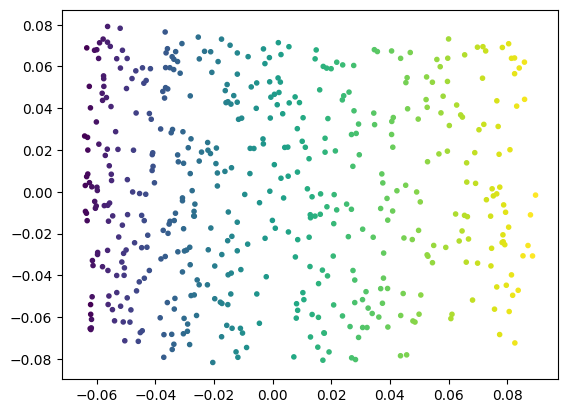
How does one perform dimensionality reduction on the Swiss roll?#
A whole class of ML methods called nonlinear dimensionality rediction has been developed specifically to work with arbitrary manifolds and structures embedded in higher dimensional spaces. We can use one example of these methods, locally-linear embedding, to learn the 2D structure of the manifold embedded in the Swiss roll dataset.
%matplotlib inline
plt.close('all')  # 3D figures sometimes need to be closed explicitly.

# Create a locally-linear embedding object; we have to tell it that our
# embedded manifold has 2 dimensions and that it should use a particular
# method called local tangent space alignment, 'ltsa'
# (see also https://en.wikipedia.org/wiki/Local_tangent_space_alignment).
lle = skl.manifold.LocallyLinearEmbedding(
    n_components=2,
    method='ltsa',
    random_state=random_state)

# Train the model on the Swiss roll points.
lle.fit(points)

# We can now use the transform method to produce 2D values:
points_2d = lle.transform(points)

# we can plot them and color them according to their manifold
# surface distance now.
(fig,ax) = plt.subplots(1,1)
(x, y) = points_2d.T
ax.scatter(x, y, marker='.', c=surface_dist)

plt.show()