Prebuilt Neural Network Models

In the previous two sections we saw how to build neural networks from scratch in PyTorch. Although these networks that we built were surprisingly capable of modeling handwritten digits, they have many drawbacks, including the amount of work required to understand what they are doing and how they work. In general, neural networks have a reputation as being “black boxes,” meaning that they are hard to understand—they are a black box that performs computations but that don’t let us see how the computations are performed inside.

In fact, the structure of CNNs and questions like “why does a certain arrangement of layers in a CNN yield especially good results?” are very hard to answer without a much deeper analysis of these techniques than this course will cover. However, there are many researchers who study neural networks specifically and who have developed network structures that excel at many kinds of problems. Many of the best model structures are not only available as existing models from PyTorch but also pre-trained on very large datasets. (Pre-trained in this case usually means that they have already been trained to recognize the content of natural images, but see the subsection on Model Generalizability below for why this matters.)

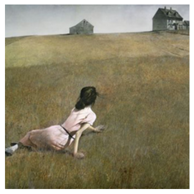
To show how these models work, we’ll want a single example image that we can pass to each model. The image doesn’t necessarily need to be classified well or correctly, but it should show how each model works, generally. We’ll use a cropped version of the painting Christina’s World by Andrew Wyeth that has been rescaled to be \(224 \times 224\) pixels; \(224 \times 224\) is a size used by many image recognition models.

import torch
import matplotlib.pyplot as plt

# Read in the image as a NumPy array:
image = plt.imread('christinas-world_cropped.png')

# Make a plot of the image so that we can see it:
plt.imshow(image)
plt.axis('off')

# Convert it into a tensor:
image = torch.from_numpy(image)
# Transpose the channels to the first dimension and add a singleton dimension
# as the batch size so that it's ready for input to a PyTorch model.
image = torch.permute(image, (2,0,1))[None, ...]

plt.show()

Prebuilt Versus Pretrained Models

There is a subtle difference between using models that are prebuilt and models that are “pretrained”. Let’s start by defining these terms:

• A prebuilt model is a model that uses a “prebuilt model architecture,” which is just a model architecture that was designed by someone else. (“Model architecture” in this case means the layers in the model and the order of computations.) All of the model architectures discussed in the sections below are prebuilt model architectures.

• A pretrained model is a model that is prebuilt and that has also already been trained to solve a particular problem. For the CNNs discussed below this is typically an object recognition problem.

Model Generalizability: Why Do Pre-trained Models Matter?

Most image-based problems that one has to solve in science are not object recognition problems, so why would one want to use a pre-trained model? This is a good question, and an important thing to keep in mind is that CNNs, especially the CNNs discussed below, are large complex models that encode in their parameters a lot of implicit knowledge about their training dataset when they are trained. This means that CNNs that have been trained to recognize the contents of a natural image may have only been trained for that specific task, but they have learned a lot implicit information about the structure of natural images in the process—their parameters encode filters generally useful for understanding what’s in an image. While this training isn’t necessarily useful for a different problem, lots of problems can benefit from that internal understanding when they start training.

To be clear, there’s nothing that stops one from doing a little bit of training on a model then stopping, then much later doing some more training. The models you construct and publish, the models others publish, and all of the models described below, can be used as starting-points in the training of new problems with new datasets.

ResNet: Natural Image Classification

One of the most well-known models that performs classificaion is a ResNet, which is short for residual network. The term “residual” here refers to the fact that the design of the ResNet allows the model to learn the difference (or residual) between the input image and the output image at each step of the computation. The purpose of this subtle difference in design isn’t to create a more expressive model but rather to enable to model to learn more quickly during training.

ResNets, like the models below, come in a number of complexities such as resnet18, resnet34, and resnet50. Each of these models is trained to accept identical input and produce identical output, but the higher the number following the name, the more parameters there are internally. (For example, resnet18 has 11,689,512 parameters while resnet34 has 21,797,672 parameters.) More parameters means that the internal representations employed by the model can be more complex, theoretically allowing it to solve more difficult problems.

ResNets can be loaded using the torch.hub interface.

import torch
import torchvision

resnet = torch.hub.load(
    'pytorch/vision:v0.13.0', 'resnet18', 
    weights='IMAGENET1K_V1')

ResNets are image classification CNNs much like the CNNs we created in the previous section but quite a bit more complex. They take, as input, a tensor whose dimensions are (N, 3, H, W) where N is the batch size; 3 is for the red, green, and blue image channels; H is the image height; and W is the image width. (H and W are pixel counts.) As output, they produce a bank of channels, each corresponding to a particular image category. Pretrained ResNets from PyTorch use the set of 1000 categories defined by the ImageNet dataset. We can find the predicted category by finding the index of the maximum value in tensor.

output = resnet(image)
torch.argmax(output[0])

If you download the ImageNet dataset and look at its category list, you will find that category 463 corresponds to “bucket, pail” which is clearly not what our image represents. This shouldn’t be surprising, however—this painting is unlike anything that is included in ImageNet and is just intended to show how the model works. If one wanted to use a ResNet in a model that predicted a different number of output categories, one could easily map the 1000 outputs of the resnet to a different number of outputs using a torch.nn.Linear. For example, the following model uses a ResNet to categorize a 3-channel image into one of only 3 categories.

import torch

class ResNet3Categories(torch.nn.Module):
    def __init__(self, resnet='resnet18', weights='IMAGENET1K_V1'):
        self.resnet = torch.hub.load(
            'pytorch/vision:v0.13.0', resnet,
            weights=weights)
        self.reduce_outputs = torch.nn.Linear(1000, 3)
    def forward(self, inputs):
        out = self.resnet(inputs)
        out = self.reduce_outputs(out)
        return out

DenseNet: A Variant of ResNet

DenseNet is a model that is similar to ResNet but with fewer parameters. Internally, a DenseNet121 contains 7,978,856 parameters, substantially fewer than the simplest ResNet (ResNet18). However, DenseNet has substantially more complex reuse of its hidden (internal) features, and this can sometimes result in longer training times.

model = torch.hub.load(
    'pytorch/vision:v0.13.0', 'densenet121',
    weights='IMAGENET1K_V1')

output = model(image)
torch.argmax(output[0])

Notice that DenseNet predicts the same “bucket, pail” category that ResNet predicts! Both models are high-performing models that were trained on the same dataset in this case, so this shouldn’t be all that surprising either. Both models are likely to have similar interpretations of images and biases.

Segmentation Networks

All of the models described above are models that perform classification—that is, determining the class or category that is represented in an image. Segmentation networks determine which pixels in an image are part of a particular object. Segmentation networks are extremely useful in a variety of image-based disciplines such as MRI and astronomy, where, for example, figuring out which parts of an image belong to a particular anatomical structure can be very time-consuming.

One common segmentation CNN is a U-Net. Unfortunately there are no official releases of U-Nets on torch.hub as of when this lesson was written. The original paper can be found at DOI: 10.48550/arXiv.1505.04597, and numerous implementations can be found online, but these have not necessarily been vetted by anyone.