Convolutional Neural Networks#
Convolutional Neural Networks (CNNs) are incredibly powerful AI/ML tools whose design resembles that of the human visual system. CNNs have demonstrated an almost uncanny ability to classify natural images (i.e., images of the physical world as opposed to computer generated images such as an image of black and white stripes) and to segment distinct objects from the rest of an image. These are not the only tasks that CNNs are capable of performing, but these tasks are useful for understanding the behavior of CNNs because they are the tasks on which most other methods fail but CNNs excel.
In terms of the engineering, CNNs are highly similar to other neural network models, and we will see in this section that the definition and training of a CNN it is largely identical to the definition and training the neural network model in the previous section, with the exception of a few computational layers in the model itself.
Before we define our model and start training, however, let’s discuss what exactly a CNN is, and why CNNs are different than the feedforward networks we saw previously.
What are convolutional neural networks?#
Fundamentally, CNNs are just feedforward neural networks (FNNs) that have a particular kind of connectivity structure between layers that both makes them more efficient than a traditional FNN and gives them substantial power at classification and segmentation tasks. This structure was in fact inspired by the structure of the human visual system. In theory, one could build a traditional FNN that learned to perform the same computations as a CNN; however, the FNN would need many many more parameters to represent the same computation as a CNN. This is because CNNs can exploit an operation called convolution, which can be performed relatively quickly over an entire image.
What is convolution?#
Image convolution is an operation in which two images slide past each other and their overlap (technically, the sum of their dot products) are calculated at every overlapping position. Convolution typically uses an input image and a kernel (both of which are in fact images). The kernel is usually but not always smaller than the input iamge, and we consider the kernel to be the image that slides along the input.
The following animaged GIF demonstrates how convolution works conceptually.
Image credit: Michael Plotke, CC, via Wikimedia Commons
The image above shows a 2D image convolution for a 2D image with only 1 channel (typically a grayscale image). However, convolution can be generalized to all kinds of objects:
The convolution of two vectors is similar to the convolution of images, but there’s only one dimension for the vectors to slide along.
The convolution of two continuous functions \(f(t)\) and \(g(t)\) can be defined by integration: \((f \circledast g)(t):=\int_{-\infty}^{\infty} f(\tau) g(t-\tau) d \tau\). This can also be generalized to any number of dimensions.
Convolution can also be defined over objects with structures unrelated to images, such as graphs (see, for example graph neural networks).
Convolution can be seen as a way of applying filters to an image. For example, the following image kernels can be applied to an input image to produce variants of the original image (filtered images).

The basic idea behind a CNN is that it is a FNN whose weights are stored as image kernels instead of as matrices that express the connectivity of every input dimension to every hidden or output dimension. In a CNN, the kernel contains weights that are applied to each location in the input image to produce the output image. This allows the CNN to efficiently apply a small filter to every location in an image. In the next layer of the network, a new kernel can be applied to the output of the previous layer, allowing more complex filters to form.
Importantly, the convolution of images with multiple channels is also straightforward to define. With multiple channels, we can imagine that the input image in the above animation has multiple channels, such as 3 image channels for red, green, and blue. In such a case, we could define our kernel to also have 3 image channels, and our dot products could be calculated over all three image channels, with the kernel sliding only over the rows and columns. This would produce a single output layer, so to produce multiple output layers, we would need multiple kernels, each of which has the same number of channels as the input image. This means that output image channels are formed of combinations of the data across channels in the input, but each pixel in the output image aggregates information from a localized section of the input image.
In the above examples, all of the kernel images are small \(3 \times 3\) images. A kernel needn’t be this small, but in convolutional neural networks, most of the kernels tend to be \(7 \times 7\) kernels or smaller. Additionally, all of the kernels in the above examples were applied to every pixel of the input image. Sometimes, CNNs will skip over every other pixel as a way to downsample the input image into a smaller image. This operation is often accompanied by the addition of channels to the output image—i.e., a convolution will convert an input whose shape is (N, C, H, W) into an output whose shape is (N, C_new, H_new, W_new) where H_new < H and W_new < W (for image height H and width W) but C_new > C (channels).
Building a CNN for the MNIST Dataset#
Let’s go ahead and build a CNN, based on our FNN from the previous section, to predict digits from the MNIST dataset. We can start by loading in the MNIST dataset.
from torchvision.datasets import MNIST
from torchvision.transforms import ToTensor
from pathlib import Path

train_dset = MNIST(Path.home(), download=True, train=True, transform=ToTensor())
test_dset = MNIST(Path.home(), download=True, train=False, transform=ToTensor())
Once we’ve loaded in the dataset, we can go ahead and define our CNN. The CNN is similar to the FNN code, but we will use slightly different layers in our CNN. We’ll add convolutional layers using PyTorch’s Conv2d class, which represents a 2D convolution applied to an image. Like other PyTorch model layers, it expects the inuput to begin with the dimensions (N,C) (batches and channels), and will generally just work if we respect this convention.
import torch

class CNNModel(torch.nn.Module):
    "A simple convolutional neural network model for the MNIST dataset."
    def __init__(self,
                 input_channels=1,
                 output_channels=10):
        super().__init__()
        # We'll start with a convolution of the input followed by a ReLU.
        # Note that this convolution will cut 1 pixel off of each border
        # because by default PyTorch's image convolution throws away pixels
        # where some of the kernel hangs off of the edge of the image.
        self.conv1 = torch.nn.Conv2d(
            in_channels=input_channels,
            # We won't change the number of output channels here:
            out_channels=input_channels,
            # We want a kernel that is 3x3 pixels:
            kernel_size=3)
        self.relu1 = torch.nn.ReLU()
        # After these operators, our image will be 26x26 instead of 28x28.
        # Next, we'll do another convolution, but one that downsamples the
        # image using the stride option, which tells the convolution how
        # many pixels to skip over when it performes the convolution.
        self.conv2 = torch.nn.Conv2d(
            in_channels=input_channels,
            # We'll increase the number of channels in this convolution:
            out_channels=(2 * input_channels),
            # Our kernel will be 7x7 this time:
            kernel_size=7,
            stride=2)
        self.relu2 = torch.nn.ReLU()
        # We'll repeat this downsampling operation a couple of times:
        self.conv3 = torch.nn.Conv2d(
            in_channels=(2 * input_channels),
            out_channels=(4 * input_channels),
            kernel_size=7,
            stride=2)
        self.relu3 = torch.nn.ReLU()
        # After downsampling twice, we should have 4 input channels but it's
        # a bit unclear how big the images should be in terms of rows and cols
        # because of our downsampling and border removal. We could count the
        # correct number of channels, rows, and columns at this point, but
        # there's also a special kind of fully-connected linear neural network
        # layer that will figure out the number of inputs for us:
        self.final = torch.nn.LazyLinear(out_features=10)
    def forward(self, inputs):
        # Notice that for convolutional neural networks, we don't reshape or
        # flatten our inputs; the convolution layers need the image to still
        # be organized as an image.
        out1 = self.conv1(inputs)
        out1 = self.relu1(out1)
        out2 = self.conv2(out1)
        out2 = self.relu2(out2)
        out3 = self.conv3(out2)
        out3 = self.relu3(out3)
        output_flat_shape = (inputs.shape[0], 1, -1)
        output = self.final(torch.reshape(out3, output_flat_shape))
        return output[:, 0]
    def predict(self, inputs):
        """Returns the integer digit prediction for the given input tensor.

        This model's outputs are a 10-element tensor in which each of the 10
        dimensions represents one digit; the dimension with the highest value
        indicates the model's predicted digit. This function runs the model on
        an input and translates the model's output into a digit.
        """
        outputs = model(inputs)
        # Keep in mind there will be a batch dimension for inputs and outputs.
        digits = torch.argmax(outputs, dim=-1)
        return digits.to(torch.uint8)

model = CNNModel()
model
CNNModel(
  (conv1): Conv2d(1, 1, kernel_size=(3, 3), stride=(1, 1))
  (relu1): ReLU()
  (conv2): Conv2d(1, 2, kernel_size=(7, 7), stride=(2, 2))
  (relu2): ReLU()
  (conv3): Conv2d(2, 4, kernel_size=(7, 7), stride=(2, 2))
  (relu3): ReLU()
  (final): LazyLinear(in_features=0, out_features=10, bias=True)
)
Training our first CNN#
Training our CNN is almost identical to training our FNN; the only real difference here is that we will use our new CNNModel class instead of the FNN model we defined in the last section.
# Hyperparameters:
n_epochs = 5       # 1 epoch: you show all your training data to your model once
lr = 0.001         # We use a fairly low learning rate.
batch_size = 1000  # How many images in one training batch.

# Make the model:
model = CNNModel()

# Make the optimizer:
optimizer = torch.optim.Adam(model.parameters(), lr=lr)

# Declare our loss function:
loss_fn = torch.nn.CrossEntropyLoss(reduction='sum')

# Make the dataloaders:
train_dloader = torch.utils.data.DataLoader(train_dset, batch_size=batch_size, shuffle=True)
test_dloader = torch.utils.data.DataLoader(test_dset, batch_size=batch_size, shuffle=True)

# Now we start the optimization loop:
for epoch_num in range(n_epochs):
    # Put the model in train mode:
    model.train()
    # In each epoch, we go through each training sample once; the dataloader
    # gives these to us in batches:
    total_train_loss = 0
    for (inputs, targets) in train_dloader:
        # We're starting a new step, so we reset the gradients.
        optimizer.zero_grad()
        # Calculate the model prediction for these inputs.
        preds = model(inputs)
        # Calculate the loss between the prediction and the actual outputs.
        train_loss = loss_fn(preds, targets)
        # Have PyTorch backward-propagate the gradients.
        train_loss.backward()
        # Have the optimizer take a step:
        optimizer.step()
        # Add up the total training loss:
        total_train_loss = total_train_loss + train_loss
    mean_train_loss = (total_train_loss / len(train_dset)).detach()
    # Now that we've finished training, put the model back in evaluation mode.
    model.eval()
    # Evaluate the model using the test data.
    total_test_loss = 0
    for (inputs, targets) in test_dloader:
        preds = model(inputs)
        test_loss = loss_fn(preds, targets)
        total_test_loss = total_test_loss + train_loss
    mean_test_loss = (total_test_loss / len(test_dset)).detach()
    # Print something about this step:
    print(f"Epoch {epoch_num:2d}:"
          f"  train loss={mean_train_loss:6.3f};"
          f"  test loss={mean_test_loss:6.3f}")
# After the optimizer has run, print out what it's found:
print("Final result:")
print(f"  train loss = ", float(mean_train_loss))
print(f"   test loss = ", float(mean_test_loss))
Epoch 0: train loss= 2.308; test loss= 2.301
Epoch 1: train loss= 2.115; test loss= 1.695
Epoch 2: train loss= 1.119; test loss= 0.792
Epoch 3: train loss= 0.733; test loss= 0.705
Epoch  4:  train loss= 0.636;  test loss= 0.588
Final result:
  train loss =  0.6364573836326599
   test loss =  0.5875511169433594
Clearly out training was successful in that the model performed better as the training went on, both on the training and the test dataset. However, the accuracy achieved was not as high as it was for the FNN in the previous section. This is partly because, despite the apparent complexity of the convolution operator, we have defined a very simple neural network. In fact, our CNN has only 676 parameters. The final FNN we built in the previous section had 1,863,690 parameters! On some level, the most surprising thing about this is how well our CNN does given that the FNN has almost 3000 times as many parameter dimensions!
Note
We can calculate the number of parameters (dimensions) in a model by extracting the individual parameter tensors and counting up the number of elements in each. The parameter tensors can be obtained via the model.parameters() method:
# Note that we have to convert the tensor shapes and products into tensors
# themselves in order use them with PyTorch functions like `prod`.
n_params = sum(
    [torch.prod(torch.tensor(param_tens.shape))
     for param_tens in model.parameters()])
Additionally, although we have included some rectified linear unit (ReLU) layers to act as activation functions, there are a number of additional layers that are known to be effective for convolutional neural networks specifically that we haven’t used. Let’s look at a couple of examples of these:
Max pooling layers. Max pooling layers divide the image up into a number of sub-images and select the maximum pixel value (usually within a channel) of the sub-images. This operation is a way of allowing the network to aggregate computations over subportions of the image. The following image shows an example of how max pooling works.
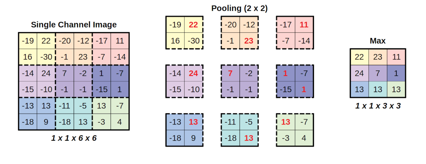
Image credit: Daniel Voigt Godoy, CC-BY-4, via Wikimedia Commons
Layer normalization layers. There are a number of ways to normalize the input and hidden layers of a CNN; normalization can occur across channels, across batches, across feature dimensions, or any other combination of these. We will not discuss all the possible ways to normalize CNN data, but one of the most common kind of normalization in CNNs is layer noralization, in which each observation in the batch is normalized independently.
Let’s try to build a CNN using these new tools then try training it again.
class ComplexCNNBlock(torch.nn.Module):
    "A single component of our complex CNN."
    def __init__(self, input_channels):
        super().__init__()
        # Each block
        self.conv1 = torch.nn.Conv2d(
            in_channels=input_channels,
            out_channels=(4*input_channels),
            kernel_size=3,
            # By providing padding=1, we prevent the erosion of the input by
            # 1 pixel along each border when we convolve.
            padding=1)
        self.relu = torch.nn.ReLU()
        self.conv2 = torch.nn.Conv2d(
            in_channels=(4*input_channels),
            out_channels=(4*input_channels),
            kernel_size=3,
            padding=1)
        # We make a MaxPool analysis that pools over 2x2 patches:
        self.maxpool = torch.nn.MaxPool2d(2)
    def forward(self, inputs):
        out = self.conv1(inputs)
        out = self.relu(out)
        out = self.conv2(out)
        return self.maxpool(out)

class ComplexCNNModel(torch.nn.Module):
    "A more complex convolutional neural network model for the MNIST dataset."
    def __init__(self,
                 input_channels=1,
                 output_channels=10):
        super().__init__()
        # We'll start with a layer norm operation to make sure our inputs are
        # normalized; we provide the input [28, 28] to indicate that we want
        # to normalize over the last 2 dimensions.
        self.input_norm = torch.nn.LayerNorm([28, 28])
        # Next, we'll have four of our ComplexCNNBlocks:
        self.block1 = ComplexCNNBlock(input_channels)
        self.block2 = ComplexCNNBlock(4 * input_channels)
        self.block3 = ComplexCNNBlock(16 * input_channels)
        self.final = torch.nn.LazyLinear(out_features=10)
    def forward(self, inputs):
        inputs = self.input_norm(inputs)
        output = self.block1(inputs)
        output = self.block2(output)
        output = self.block3(output)
        output = self.final(torch.reshape(output, (inputs.shape[0], 1, -1)))
        return output[:, 0]
    def predict(self, inputs):
        """Returns the integer digit prediction for the given input tensor.

        This model's outputs are a 10-element tensor in which each of the 10
        dimensions represents one digit; the dimension with the highest value
        indicates the model's predicted digit. This function runs the model on
        an input and translates the model's output into a digit.
        """
        outputs = model(inputs)
        # Keep in mind there will be a batch dimension for inputs and outputs.
        digits = torch.argmax(outputs, dim=-1)
        return digits.to(torch.uint8)

model = ComplexCNNModel()
model
ComplexCNNModel(
  (input_norm): LayerNorm((28, 28), eps=1e-05, elementwise_affine=True)
  (block1): ComplexCNNBlock(
    (conv1): Conv2d(1, 4, kernel_size=(3, 3), stride=(1, 1), padding=(1, 1))
    (relu): ReLU()
    (conv2): Conv2d(4, 4, kernel_size=(3, 3), stride=(1, 1), padding=(1, 1))
    (maxpool): MaxPool2d(kernel_size=2, stride=2, padding=0, dilation=1, ceil_mode=False)
  )
  (block2): ComplexCNNBlock(
    (conv1): Conv2d(4, 16, kernel_size=(3, 3), stride=(1, 1), padding=(1, 1))
    (relu): ReLU()
    (conv2): Conv2d(16, 16, kernel_size=(3, 3), stride=(1, 1), padding=(1, 1))
    (maxpool): MaxPool2d(kernel_size=2, stride=2, padding=0, dilation=1, ceil_mode=False)
  )
  (block3): ComplexCNNBlock(
    (conv1): Conv2d(16, 64, kernel_size=(3, 3), stride=(1, 1), padding=(1, 1))
    (relu): ReLU()
    (conv2): Conv2d(64, 64, kernel_size=(3, 3), stride=(1, 1), padding=(1, 1))
    (maxpool): MaxPool2d(kernel_size=2, stride=2, padding=0, dilation=1, ceil_mode=False)
  )
  (final): LazyLinear(in_features=0, out_features=10, bias=True)
)
# Hyperparameters:
n_epochs = 5       # 1 epoch: you show all your training data to your model once
lr = 0.001         # We use a fairly low learning rate.
batch_size = 1000  # How many images in one training batch.

# Make the model:
model = ComplexCNNModel()

# Make the optimizer:
optimizer = torch.optim.Adam(model.parameters(), lr=lr)

# Declare our loss function:
loss_fn = torch.nn.CrossEntropyLoss(reduction='sum')

# Make the dataloaders:
train_dloader = torch.utils.data.DataLoader(train_dset, batch_size=batch_size, shuffle=True)
test_dloader = torch.utils.data.DataLoader(test_dset, batch_size=batch_size, shuffle=True)

# Now we start the optimization loop:
for epoch_num in range(n_epochs):
    # Put the model in train mode:
    model.train()
    # In each epoch, we go through each training sample once; the dataloader
    # gives these to us in batches:
    total_train_loss = 0
    for (inputs, targets) in train_dloader:
        # We're starting a new step, so we reset the gradients.
        optimizer.zero_grad()
        # Calculate the model prediction for these inputs.
        preds = model(inputs)
        # Calculate the loss between the prediction and the actual outputs.
        train_loss = loss_fn(preds, targets)
        # Have PyTorch backward-propagate the gradients.
        train_loss.backward()
        # Have the optimizer take a step:
        optimizer.step()
        # Add up the total training loss:
        total_train_loss = total_train_loss + train_loss
    mean_train_loss = total_train_loss.detach() / len(train_dset)
    # Now that we've finished training, put the model back in evaluation mode.
    model.eval()
    # Evaluate the model using the test data.
    total_test_loss = 0
    for (inputs, targets) in test_dloader:
        preds = model(inputs)
        test_loss = loss_fn(preds, targets)
        total_test_loss = total_test_loss + train_loss
    mean_test_loss = total_test_loss.detach() / len(test_dset)
    # Print something about this step:
    print(f"Epoch {epoch_num:2d}:"
          f"  train loss={mean_train_loss:6.3f};"
          f"  test loss={mean_test_loss:6.3f}")
# After the optimizer has run, print out what it's found:
print("Final result:")
print(f"  train loss = ", float(mean_train_loss))
print(f"   test loss = ", float(mean_test_loss))
Epoch 0: train loss= 1.069; test loss= 0.346
Epoch 1: train loss= 0.217; test loss= 0.149
Epoch 2: train loss= 0.116; test loss= 0.117
Epoch 3: train loss= 0.084; test loss= 0.048
Epoch  4:  train loss= 0.068;  test loss= 0.067
Final result:
  train loss =  0.06796513497829437
   test loss =  0.06653345376253128
While the exact loss value that your network achieves will depend on random factors, such as the random initial values assigned to the model parameters, hopefully it is clear that this version of the network worked quite a bit better than the previous version and is roughly comparable with the model that we produces in the previous section. We substantially increased the complexity of each convolutional layer this time by adding many additional output channels. This model has a 56,646 dimensions in its parameter-space, making it substnatially larger than our first model, but still only about 5% of the size of our FNN model.