What is Supervised Learning?#
A common use of data is to make a model. Typically when one makes a model, one uses some features of a dataset to predict other features. For example, one might make a model using the California Housing Dataset that predicts the median houshold income of an area from other factors like the median age and size of houses in the area. Sometimes one has a particular model form in mind and simply wants to fit its parameters (see Lesson 3); other times one doesn’t especially care what the form of the model is. This lesson surveys a number of these latter methods. In both cases, supervised learning is usually called for.
Put simply, supervised learning methods learn to make predictions by examining correct examples of associations between their inputs and their outputs (often with some amount of noise in the examples). This general method is also how humans learn: estimating the number of microliters of liquid in a tiny drop of water is a very difficult task, but biochemists who use micropipettes daily usually get very good at this task. This isn’t because they consciously adopt a specific algorithm but because they are exposed to enough examples that they learn the association organically.
While the AI/ML methods we will discuss in this section do not learn “organically” in the same way that animals do, they are applicable to many kinds of datasets, and they are generally agnostic regarding the specific structure of a dataset or the underlying theories/models that give rise to it.
Lesson Goals#
In this lesson we will learn what we can about the California Housing dataset by training models using examples from the dataset. By the end of this lesson, you should be comfortable with the following concepts and methods.
We’ll start by discussing a few core concepts: training, regression/classification, overfitting, and cross validation.
We’ll then discuss linear regression, one of the most important and interpretable supervised learning methods.
Next, we’ll discuss random forests, a less interpretable but very robust and flexible method.
Finally, we’ll look at support vector machines, one of the most well-studied methods in ML.
Supervised Learning Concepts#
Training and Evaluation#
Unlike the unsupervised learning methods we saw in the previous section, supervised learning methods need to be trained before they work. During training, the model is repeatedly updated to improve its ability to predict output values. Once it has been trained, it can be evaluated to predict the output for any valid input value, even values that it was not shown during training.
In order to train and evaluate a method, we need a metric for measuring how accurate or inaccurate a method’s predictions are. We call this metric a loss function. A loss function typically takes the form \(l(y, \hat{y})\) where \(y\) is a measurement or observation in a dataset and \(\hat{y}\) is a prediction of the model. A higher loss indicates more error in the model’s predictions—in fact, the goal of most supervised methods is to minimize a loss function (though different methods use different loss functions). There are many loss functions, but a very common example is the quadratic loss: \(l(y, \hat{y}) = (y - \hat{y})^2\).
Regression versus Classification#
In the previous lesson on Unsupervised Learning, we saw how different unsupervised methods perform different kinds of operations; K-Means is a clustering algorithm whereas PCA is a dimensionality reduction algorithm. Supervised methods broadly fall into two categories: regression methods and classification methods.
Regression is the prediction of a continuous value from a set of example data. Linear regression, which we will look at in the next section, is the most common type of regression, but many other methods such as Random Forests, perform similar operations.
Classification is the prediction of a category or class for a given input. For example, convolutional neural networks that are capable of labeling the contents of an image are classification models.
In many cases, regression methods and classification methods are solved by nearly identical algorithms. For example, a linear regression model can learn a linear relationship between input values (x) and output values (y) by examining many examples of (x, y) pairs. Once it has learned the relationship, it can predict a real number y that goes with an input x, even if it has never seen that input during training. Suppose, however, that instead of being given real numbers for y, every y value was either a 0 or a 1 (i.e., every x was either a member or not a member of a particular class). In this case, we could train the model to produce a real number but interpret the value as a 0 when y < 0.5 and as a 1 otherwise. In fact, logistic regression is a variant of linear regression used for classification.
Overfitting and Cross Validation#
When one trains a supervised model using real data there is always the problem of overfitting. Overfitting occurs when a model is trained so well on one dataset that it can’t perform well on a similar dataset. This may sound unintuitive, so let’s consider an example.
Suppose one were given the following dataset and asked to construct a model of it.
import numpy as np
import matplotlib.pyplot as plt

# Our dataset will consist of only 4 (x,y) points:
x = [0,    0.20, 0.80, 2.05, 3]
y = [0.16, 0.05, 1.18, 1.73, 2.88]

# We can plot them to visualize them:
plt.plot(x, y, 'ko')

# We can also plot a reference line of x=y:
plt.plot([0,3], [0,3], 'r:')

plt.show()
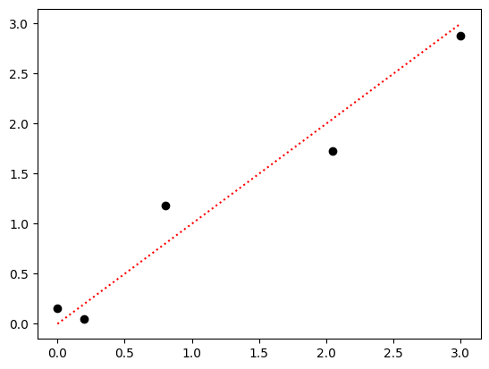
Clearly, these points approximately form a unity line with a small amount of noise in the precise measurements. If someone asked you to predict the correct value for x = 1.5, your best prediction would probably be very close to 1.5.
However, if we didn’t plot or examine the points and simply wanted to find the most accurate model possible, one might try to fit a degree 4 polynomial to the points. Degree 4 polynomials are those of the form \(c_4 x^4 + c_3 x^3 + c_2 x^2 + c_1 x + c_0 = 0\). We won’t discuss the details of how one fits such a model in this course, but the numpy library includes a function, polyfit that will find the parameters \(c_0\), \(c_1\), \(c_2\), \(c_3\), and \(c_4\) for us.
# Find the polynomial coefficients:
(c4, c3, c2, c1, c0) = np.polyfit(x, y, deg=4)

# Make a function that calculates the polynomial prediction:
def f(x):
    return c4*x**4 + c3*x**3 + c2*x**2 + c1*x + c0

# Let's replot the data with this function!
plt.plot(x, y, 'ko')

# Plot the polynomial:
x_tmp = np.linspace(0, 3, 100)
y_tmp = f(x_tmp)
plt.plot(x_tmp, y_tmp, 'c:')

plt.show()
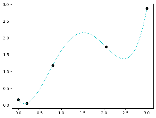
This may look like a good estimate, in that the model prediction exactly predicts each of the input points. However, when asked what the predicted value for 2.5 is, the result is not all that close to 2.5:
print(f(2.5))
1.376407869617108
In this example, the 4th-degree polynomial model is highly accurate when predicting the training data—i.e., any of the data used to train the model. However, when predicting data that is not part of the traning data, the model will perform poorly. This phenomenon indicates that the model is overfit.
An even more egregious example can be found by increasing the number of data points and the degree of the model. Here’s an example using 10 data points that are approximately on the line of unity, fit using a degree 9 polynomial.
# The x values are just 0–9:
x = np.arange(10)
# The y-values are the same with a little normally-distributed noise:
y = x + np.random.randn(10)

# Fit the points:
coefficients = np.polyfit(x, y, deg=9)

# Make a function that calculates the polynomial prediction:
def f(x):
    return np.sum(
        [c * x**k for (k,c) in enumerate(reversed(coefficients))],
        axis=0)

# Plot the data:
plt.plot(x, y, 'k.')
x_tmp = np.linspace(0, 9, 500)
plt.plot([0,9], [0,9], 'r:')
plt.plot(x_tmp, f(x_tmp), 'c:')
plt.ylim([-5,15])

plt.show()
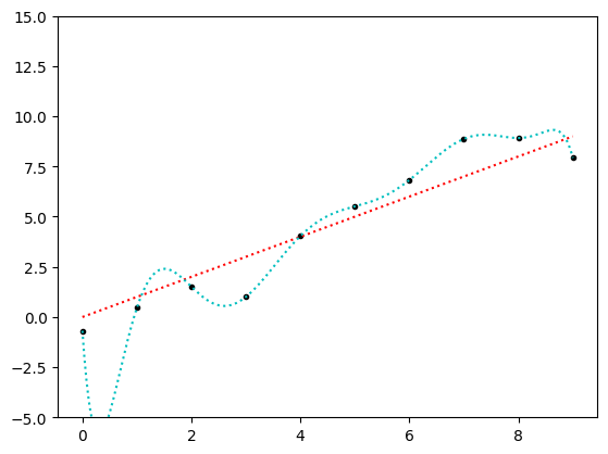
Clearly the above model is highly overfit: it is very unlikely that the true process that generated these data points varies as much between the measured points as the cyan curve does in this plot. But the cyan curve goes through every point in the dataset exactly. If all we cared about was minimizing the error of all of our measurements relative to our model, then the cyan is objectively better. However, if we care about how well our model would predict a new measurement not already in the dataset, the cyan curve will perform poorly.
The problem of how to avoid overfitting is substantial, and many different kinds of strategies exist. However, the most useful and common strategy is appropriate for most model-fitting scenarios: cross validation. Using cross validation is straightforward; the basic idea involves three steps:
Split the dataset into at least two subdatasets, the training data and the test data; no data point should appear in both datasets (even if the dataset contains duplicate identical data points).
Train the model using the training data.
Evaluate the model’s accuracy using the test data.
This strategy ensures that when you test your model, you don’t test it on data that it might be overfit to. For example, in the previous cell we could have removed three of the points at random (test data), fit the polynomial or the line to the remaining seven points (training data), then evaluated how well the polynomial or line predicted the three test points. Most likely, the line would fit the test points quite well while the polynomial will have been overfit to the training data and would fit the three test points quite poorly.
Cross validation has many variants that all use this basic strategy. For example, sometimes a dataset is split into \(k\) distinct subdatasets then each of the subdatasets is used as a test dataset for a model trained using all the remaining subdatasets. Typically, one makes a test dataset that is much smaller than the training dataset because it takes a lot of data to train most models, but relatively little data to evaluate one.
Parameters, Inputs, Outputs, and Hyperparameters#
Models have parameters, which are configurable variables that allow the model to take different forms. When we fit a model to data, what we actually do is change the parameters such that the model’s form best explains the data. Parameters are different than the model’s inputs, which are the values used to train and evaluate the model. Inputs are also frequently called features. In the example above in which we fit a 4th degree polynomial to a set of points using numpy.polyfit, the values \(c_0\), \(c_1\), \(c_2\), \(c_3\), and \(c_4\) are the parameters of the model, which we fit from the examples of (x,y) points. Those points make up the model’s inputs (x) and outputs (y), which are also sometimes called targets. Given a different set of points, the numpy.polyfit function would have returned a different set of model parameters that would represent a different form of the model (a polynomial with a different shape).
Models with more parameters are generally more complex and thus more able to model a wider variety of data. For example, the model \(f(x; m) = m \, x\), where \(x\) is the model’s input and \(m\) is a single parameter, is able to accurately model a lot more kinds of data (any line that goes through the origin) than the simpler model \(g(x; m) = m\), which can model only horizontal lines.
Additionally, models have hyperparameters. A hyperparameter is a value that does not appear in the formal model but that was used in its training. For example, some models are trained by viewing the training samples in a sequence and updating the model parameters after each sample. For such a model, the order in which the samples are shown to the model is a hyperparameter. It may have an effect on the final model parameters, but it isn’t part of the model itself. As we go through the methods in this section, we will discuss the hyperparameters involved in training them alongside the details of the methods themselves. When a method has many hyperparameters, it can be important to use additional layers of cross validation, which we will discuss in Lesson 3.
The Bias / Variance Tradeoff#
In this section, we consider a variety of supervised learning models, each of which has a set of internal parameters. The models are each trained using a dataset containing examples of model inputs paired with correct outputs, both of which can contain noise. When we train a model, the noise inherent in the dataset contributes to the irreducible error: noise that cannot be explained because it is inherently noise and not signal. If we train a model using any particular dataset, which in the real world will always contain noise, how well the model performs will in part depend on the model’s complexity. If the model is very simple, then, after training, it is more likely to exhibit bias, meaning that it adheres to its assumptions rather than the data on which it was trained. Such a model is underfit. On the other hand, a complex model is likely to exhibit variance, which has a slightly different meaning in this context than that of “the variance of a dataset”. In this context, the variance refers to a complex model’s ability to fit data so well that it even fits the noise. Such a model is overfit. In our earlier example, the 4th degree polynomial perfectly fit the noise in the measurements and thus was exhibiting high variance.
In general, there is a tradeoff between the bias of a model and its variance. For a given dataset, a very simple model like the model \(f(x; m) = m\) we saw earlier will exhibit bias. If we make the model slightly more complex, such as \(h(x; m, b) = m \, x + b\), and fit that model to the same dataset, the model becomes slightly more likely to exhibit variance. If the dataset actually measured a constant value with respect to \(x\), just with some noise in each measurement (i.e., the model \(f\) is closer to the truth in this case), then it is likely that the model \(h\) will find a small non-zero parameter for \(m\) due to noise.
The more complex the model, the mode likely it is to exhibit variance, but the appropriate model complexity is different for every problem and often must be determined experimentally by fitting several models of different complexity. In such cases, starting with the simplest plausible model and progressively testing more complex models using cross validation is a good general approach.